It is well known that adult male heights follow a normal (Gaussian) distribution. The same is true of adult female heights. But what does the distribution of heights look like for adults in general? You might be surprised.
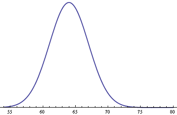
Assume heights for women follow a normal distribution with mean of 64 inches and standard deviation 3 inches.
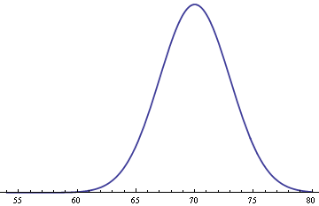
Assume men’s heights follow the same distribution but with an average of 70 inches.
Finally, assume men and women each make up 50% of the population. Then you get the following distribution for the heights of adults in general.
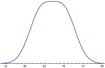
The mixture is surprisingly flat on top. Minor variations on the assumptions above can change the shape, making it more rounded at the top, making it dip in the middle, or making it tip to one side.
See Adult heights and mixture distributions for mathematical details.
See also Why heights are normally distributed.
Beautiful post. Mostly because it shows that heights does not follow a normal distribution. Ah! Ah!
Thanks. I expected a bimodal density, so I was surprised when it came out flat on top. I suppose my expectations were backward: bimodal distributions are often mixtures, so I expected my mixture would be bimodal. With a slight change in assumptions it is bimodal, but not strongly so, still essentially flat on top.
See also this recent paper in The American Statistician:
Is Human Height Bimodal?
Mark F. Schilling, Ann E. Watkins and William Watkins
The American Statistician, Vol. 56, No. 3 (Aug., 2002), pp. 223-229
http://www.jstor.org/stable/3087302
Thanks! I didn’t know about that article.
Like the article says, this is the canonical example of a bimodal distribution. I mentioned it in passing as an example a few days ago in a class I’m teaching. When I sat down to make some plots to take to the next class I found out I was wrong.
Deb Nolan and I discuss this example in our Teaching Statistics book from 2002. We display a density curve which, as it happens, is neither bimodal nor flat on top. The distribution for men has a slightly higher variance. I agree that this is a good classroom example.
A joke has it that the scientists believe is is the mathematicians who know the data to be normally distributed while the mathematicians believe is is the scientists who possess this knowledge. In logic, there is no reason for one to believe the data are normally distributed. It is the sample mean which, under widely applicable circumstances, is normally distributed.
Interesting! If we take this into a regression context, does this mean that the normal distribution assumption for the errors won’t hold if we omit a covariate? (Creating an additional problem besides potential omitted variable bias in the coefficients?)
You say in this post that the resulting distribution looks surprisingly flat, so I wanted to figure out how far the two distributions have to be apart for it to be *exactly* flat. Turns out: 2 standard distributions, exactly as is the example here.
More specificially, if you compute the 2nd derivative in x=0 of the distribution you get by creating a 50/50 mixture of a normal distribution with sigma=1 mu=-a and one with sigma=1 mu=+a, you get (a^2-1)*exp(-a^2/2)/sqrt(2*pi). This value is 0 exactly when a=1 or a=1.
This means that 50/50 mixtures of normal distributions with a shifted version of themselves result in a bimodal distribution when the shift exceeds 2 standard deviations.
Sigh, I just realized you give that exact same reasoning in your other blog post linked here about the mathematical details. Sorry!