The following definition of robust statistics comes from P. J. Huber’s book Robust Statistics.
… any statistical procedure should possess the following desirable features:
- It should have a reasonably good (optimal or nearly optimal) efficiency at the assumed model.
- It should be robust in the sense that small deviations from the model assumptions should impair the performance only slightly. …
- Somewhat larger deviations from the model should not cause a catastrophe.
Classical statistics focuses on the first of Huber’s points, producing methods that are optimal subject to some criteria. This post looks at the canonical examples used to illustrate Huber’s second and third points.
Huber’s third point is typically illustrated by the sample mean (average) and the sample median (middle value). You can set almost half of the data in a sample to ∞ without causing the sample median to become infinite. The sample mean, on the other hand, becomes infinite if any sample value is infinite. Large deviations from the model, i.e. a few outliers, could cause a catastrophe for the sample mean but not for the sample median.
The canonical example when discussing Huber’s second point goes back to John Tukey. Start with the simplest textbook example of estimation: data from a normal distribution with unknown mean and variance 1, i.e. the data are normal(μ, 1) with μ unknown. The most efficient way to estimate μ is to take the sample mean, the average of the data.
But now assume the data distribution isn’t exactly normal(μ, 1) but instead is a mixture of a standard normal distribution and a normal distribution with a different variance. Let δ be a small number, say 0.01, and assume the data come from a normal(μ, 1) distribution with probability 1-δ and the data come from a normal(μ, σ2) distribution with probability δ. This distribution is called a “contaminated normal” and the number δ is the amount of contamination. The reason for using the contaminated normal model is that it is a non-normal distribution that may look normal to the eye.
We could estimate the population mean μ using either the sample mean or the sample median. If the data were strictly normal rather than a mixture, the sample mean would be the most efficient estimator of μ. In that case, the standard error would be about 25% larger if we used the sample median. But if the data do come from a mixture, the sample median may be more efficient, depending on the sizes of δ and σ. Here’s a plot of the ARE (asymptotic relative efficiency) of the sample median compared to the sample mean as a function of σ when δ = 0.01.
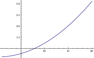
The plot shows that for values of σ greater than 8, the sample median is more efficient than the sample mean. The relative superiority of the median grows without bound as σ increases.
Here’s a plot of the ARE with σ fixed at 10 and δ varying between 0 and 1.
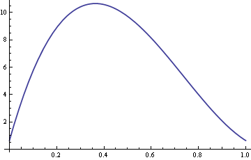
So for values of δ around 0.4, the sample median is over ten times more efficient than the sample mean.
The general formula for the ARE in this example is 2((1 + δ(σ2 – 1)(1 – δ + δ/σ)2)/ π.
If you are sure that your data are normal with no contamination or very little contamination, then the sample mean is the most efficient estimator. But it may be worthwhile to risk giving up a little efficiency in exchange for knowing that you will do better with a robust model if there is significant contamination. There is more potential for loss using the sample mean when there is significant contamination than there is potential gain using the sample mean when there is no contamination.
Here’s a conundrum associated with the contaminated normal example. The most efficient estimator for normal(μ, 1) data is the sample mean. And the most efficient estimator for normal(μ, σ2) data is also to take the sample mean. Then why is it not optimal to take the sample mean of the mixture?
The key is that we don’t know whether a particular sample came from the normal(μ, 1) distribution or from the normal(μ, σ2) distribution. If we did know, we could segregate the samples, average them separately, and combine the samples into an aggregate average: multiplying one average by 1-δ, multiplying the other by δ, and add. But since we don’t know which of the mixture components lead to which samples, we cannot weigh the samples appropriately. (We probably don’t know δ either, but that’s a different matter.)
There are other options than using sample mean or sample median. For example, the trimmed mean throws out some of the largest and smallest values then averages everything else. (Sometimes sports work this way, throwing out an athlete’s highest and lowest marks from the judges.) The more data thrown away on each end, the more the trimmed mean acts like the sample median. The less data thrown away, the more it acts like the sample mean.
Related post: Efficiency of median versus mean for Student-t distributions
i think mean , arithmetics, is fair enough 4 the median, maybe in a few (log(n)) tries :)
Interesting, #2 sounds like #3 in a well-posed problem definition:
https://en.wikipedia.org/wiki/Well-posed_problem