In applications you often want to take the maximum of two numbers. But the simple function
f(x, y) = max(x, y)
can be difficult to work with because it has sharp corners. Sometimes you want an alternative that sands down the sharp edges of the maximum function. One such alternative is the soft maximum. Here are some questions this post will answer.
- What exactly is a soft maximum and why is it called that?
- How is it related to the maximum function?
- In what sense does the maximum have “sharp edges”?
- How does the soft maximum round these edges?
- What are the advantages to the soft maximum?
- Can you control the “softness”?
I’ll call the original maximum the “hard” maximum to make it easier to compare to the soft maximum.
The soft maximum of two variables is the function
g(x, y) = log( exp(x) + exp(y) ).
This can be extended to more than two variables by taking
g(x1, x2, …, xn) = log( exp(x1) + exp(x2) + … + exp(xn) ).
The soft maximum approximates the hard maximum. Why? If x is a little bigger than y, exp(x) will be a lot bigger than exp(y). That is, exponentiation exaggerates the differences between x and y. If x is significantly bigger than y, exp(x) will be so much bigger than exp(y) that exp(x) + exp(y) will essentially equal exp(x) and the soft maximum will be approximately log( exp(x) ) = x, the hard maximum. Here’s an example. Suppose you have three numbers: -2, 3, 8. Obviously the maximum is 8. The soft maximum is 8.007.
The soft maximum approximates the hard maximum but it also rounds off the corners. Let’s look at some graphs that show what these corners are and how the soft maximum softens them.
Here are 3-D plots of the hard maximum f(x, y) and the soft maximum g(x, y). First the hard maximum:
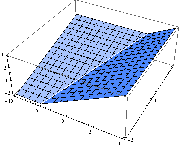
Now the soft maximum:

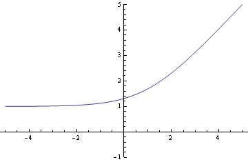
Next we look at a particular slice through the graph. Here’s the view as we walk along the line y = 1. First the hard maximum:
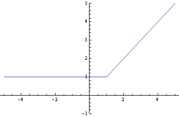
And now the soft maximum:
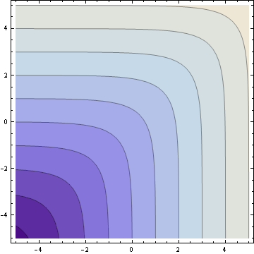
Finally, here are the contour plots. First the hard maximum:
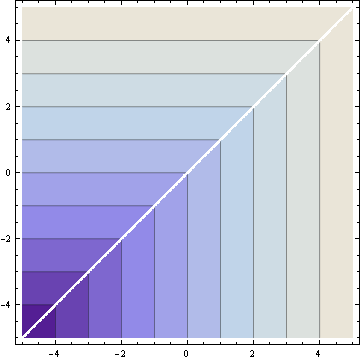
And now the soft maximum:
The soft maximum approximates the hard maximum and is a convex function just like the hard maximum. But the soft maximum is smooth. It has no sudden changes in direction and can be differentiated as many times as you like. These properties make it easy for convex optimization algorithms to work with the soft maximum. In fact, the function may have been invented for optimization; that’s where I first heard of it.
Notice that the accuracy of the soft maximum approximation depends on scale. If you multiply x and y by a large constant, the soft maximum will be closer to the hard maximum. For example, g(1, 2) = 2.31, but g(10, 20) = 20.00004. This suggests you could control the “hardness” of the soft maximum by generalizing the soft maximum to depend on a parameter k.
g(x, y; k) = log( exp(kx) + exp(ky) ) / k
You can make the soft maximum as close to the hard maximum as you like by making k large enough. For every value of k the soft maximum is differentiable, but the size of the derivatives increase as k increases. In the limit the derivative becomes infinite as the soft maximum converges to the hard maximum.
Update: See How to compute the soft maximum.
Nice find. =-)
This is actually the core of Exponential Shadow Maps technique: www-flare.cs.ucl.ac.uk/staff/J.Kautz/publications/esm_gi08.pdf
Great post!
/Tomas
Nice!
Found via your tweet.
The family of power means includes the arithmetic mean, the geometric mean, the harmonic mean, minimum, and maximum:
http://en.wikipedia.org/wiki/Power_means
By varying the exponent, you can make the “maximum” as soft or as hard as you want.
The soft maximum is a special case of the generalized f-mean:
http://en.wikipedia.org/wiki/Generalized_f-mean
What software did you use to create this graph?
http://www.johndcook.com/contoursoft.png
I really like the color palette
You’ve left out a normalization, I think, since g(x,x) = log(exp(x)+exp(x)) = log(2*exp(x)) = log(2) + x, which is not f(x,x)= x. You likely want g(x,y) = log((exp(x)+exp(y))/2), which is the Generalized f-mean that Peter Turney mentions.
Very interesting. I’m curious to know some examples of where and why you’d replace the hard maximum with the soft maximum?
Troy: one reason to replace the hard maximum with the soft maximum would be to use optimization methods (e.g. Newton’s method) that require objective functions to be twice-differentiable. I’ve also heard that the soft maximum function comes up in electrical engineering problems with power calculations.
Tim: I made my plots using Mathematica. The colors were the defaults for contour plots.
Andrew: The normalization you propose would make g(x, x) = x, which sounds like a nice property to have. But the more important property is that g(x, y) approaches max(x, y) as either argument gets large. That property would no longer hold if you included the normalization constant.
Ahh, of course. But keep y small then my g(x,y) ~ log(exp(x)/2) = x – log(2) ~ x. In either case it’s a constant difference and it’s more a question of where you want the error to go. I’m thinking more though about the region where things are sharp. In that case x and y are about the same.
Andrew: You can get a better approximation by using a different kind of normalization. See the extra parameter k in g(x, y; k) defined near the end of the post.
Yes. That’s the same approach as we did in high school to have “the equation for a square: x**N + y**N = R**N where N is very large.” But then there’s numerical problems like k=8;log(exp(98*k) + exp(101.1*k))/k overflows a IEEE double. In any case, this is a trick I’m going to keep in mind for the future, so thanks for writing about it!
Andrew: You’re right that you’d need to be careful implementing g(x, y). The intermediate computations could easily overflow even though the final value would be a moderate-sized number. A robust implementation of g(x, y) would not just turn the definition into source code. See this post for one way to compute soft maximum while avoiding overflow.
@Tim: You can also use Wolfram Alpha
http://www.wolframalpha.com/input/?i=g(x,+y)+%3D+log(+exp(x)+%2B+exp(y)+)
(someone asked about it on reddit, I can as well answer it here)
If you need a guarantee that forall_i softmax(x1,…,xn) <= xi use this function instead: softmax(x1,…xn) = log(exp(x1) + … + exp(xn)) – log(n)
Proof: log(exp(x1) + … + exp(xn)) – log(n) <= log(n * exp(xmax)) – log(n) = log(n) + log(exp(xmax)) – log(n) = log(exp(xmax)) = xmax
Derivatives identical to the function from OP. Correction term changes depending on your choice of logarithm and exponentiation base.
And yes, the function will easily overflow when naively implemented with floating point units. Computing it as xmax + softmax(x1-xmax,…,xn-xmax) trivially solves this problem, as all arguments of exponentiation will be nonpositive, and argument of the logarithm will be between 1 and n.
Very nice article. However, I was not entirely convinced that ” In the limit the derivative becomes infinite as the soft maximum converges to the hard maximum.” I wasn’t sure because the derivative on either side was finite so I was expecting the derivative to go to some finite value (based on the subgradient idea).
If my f(x)=|x|, then f(x) = max(x,-x) ~ log( exp(kx), exp(-kx) )/k. Then df/dx=tanh(kx). So when x->0 and k->inf we can make the limit go to any value but only within -1,1. Is this right?
I was wondering if you have formally published this information in any books, conferences, or journals? If so, could you please forward me the citation information so that I can read the formal papers (and any additional analysis you have done with this equation)? I think this approximation may be helpful for a research project I am just starting, however, I’d rather cite a published paper that has ideally been peer-reviewed.
Thanks!
I have not published any of this, but I could put it in a tech report and give you something to cite.
One complaint: I got a bit confused by your use of CS notation – why don’t you write “ln” when you write equations? (If these snippets were formatted as code I wouldn’t gripe, but since they’re not they should follow math conventions, right? ;P)
Charles B: The reason CS uses “log” for natural logarithm is that math does too. Unfortunately, math has two conventions. Before calculus, log may mean logarithm base 10. After calculus, log means natural log. All advanced math uses log for natural logarithm, and that’s why computer languages do too. Sorry for the confusion.
Would be good to get contributors to curate this information into wikipedia. I added a page smooth maximum, to delinate it from softMax function.
How would you cope to the problem of having nan gradient because of high k parameter ?