Where the Unix philosophy breaks down

Unix philosophy says a program should do only one thing and do it well. Solve problems by sewing together a sequence of small, specialized programs. Doug McIlroy summarized the Unix philosophy as follows.

This is the Unix philosophy: Write programs that do one thing and do it well. Write programs to work together. Write programs to handle text streams, because that is a universal interface.

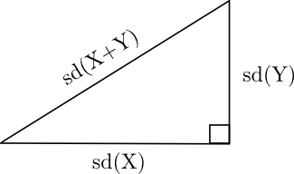
This design philosophy is closely related to “orthogonality.” Programs should have independent features just as perpendicular (orthogonal) lines run in independent directions.

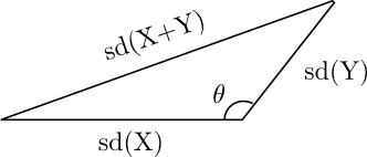
In practice, programs gain overlapping features over time.  A set of programs may start out orthogonal but lose their uniqueness as they evolve. I used to think that the departure from orthogonality was due to a loss of vision or a loss of discipline, but now I have a more charitable explanation.

The hard part isn’t writing little programs that do one thing well. The hard part is combining little programs to solve bigger problems. In McIlroy’s summary, the hard part is his second sentence: Write programs to work together.

Piping the output of a simple shell command to another shell command is easy. But as tasks become more complex, more and more work goes into preparing the output of one program to be the input of the next program. Users want to be able to do more in each program to avoid having to switch to another program to get their work done.

An example of the opposite of the Unix philosophy would be the Microsoft Office suite. There’s a great deal of redundancy between the programs. At a high level, Word is for word processing, Excel is the spreadsheet, Access is the database etc. But Excel has database features, Word has spreadsheet features, etc. You could argue that this is a terrible mess and that the suite of programs should be more orthogonal. But someone who spends most of her day in Excel doesn’t want to switch over to Access to do a query or open Word to format text. Office users are grateful for the redundancy.

Software applications do things they’re not good at for the same reason companies do things they’re not good at: to avoid transaction costs. Companies often pay employees more than they would have to pay contractors for the same work. Why? Because the total cost includes more than the money paid to contractors. It also includes the cost of evaluating vendors, writing contracts, etc. Having employees reduces transaction costs.

When you have to switch software applications, that’s a transaction cost. It may be less effort to stay inside one application and use it for something it does poorly than to switch to another tool. It may be less effort to learn how to do something awkwardly in a familiar application than to learn how to do it well in an unfamiliar application.

Companies expand or contract until they reach an equilibrium between bureaucracy costs and transaction costs. Technology can cause the equilibrium point to change over time. Decades ago it was efficient for organizations to become very large. Now transaction costs have lowered and organizations outsource more work.

Software applications may follow the pattern of corporations. The desire to get more work done in a single application leads to bloated applications, just as the desire to avoid transaction costs leads to bloated bureaucracies. But bloated bureaucracies face competition from lean start-ups and eventually shed some of their bloat or die. Bloated software may face similar competition from leaner applications. There are some signs that consumers are starting to appreciate software and devices that do less and do it well.

Related posts

Getting women to smoke

In the United States, not many women smoked before 1920. Edward Bernays, Sigmund Freud’s nephew, changed that.

Bernays’s proudest accomplishment was the creation of a nation of female tobacco addicts in the 1920s. … Bernays, who was well-connected in the media, asked photographer friends to take photos of slim, pretty women smoking. He also paid physicians to go on record stating that cigarettes were an important part of a meal because the smoke “disinfects the mouth and soothes the nerves.”

The quote above comes from the book Made by Hand by Mark Frauenfelder, editor of Make magazine. He goes on to explain other things Bernays did such as persuading restaurants to add cigarettes to the desert menu and staging public events to make it look like women smoked openly.

The campaign was quite effective.

By the end of 1928, American Tobacco’s annual revenue increased by $32 million (about $400 million in today’s money, adjusted for inflation) over the previous year.

Frauenfelder tells this story to illustrate how our desires are manipulated by advertising. Advertisers of the same era taught us “that homemade clothing was shameful, home-canned food unsanitary, and old cars symbols of failure.” Frauenfelder contends such advertising campaigns killed that America’s do-it-yourself ethic.

Related post: Smoking

Google Docs OCR

Google Docs now offers OCR (optical character recognition), but I’ve had little success getting  it to work.

The link to upload files was flaky under Firefox 3.6.4. The underlined text that says “Select files to upload” is not clickable, but you can click the white space a few millimeters above or below what looks like a link. However, the clickable white space didn’t do anything when I clicked it. The link worked just fine in IE 8 and Safari 5.0.

screen shot of page to upload documents for OCR

I clicked the check box that says “Convert text from PDF or image files to Google Docs documents” and uploaded a PDF file. The file was a decent quality scan of a paper document.

section of text from a scanned article

I got a message back saying “Unable to convert document.”

So I tried again with a PDF file that had been created from a LaTeX file using pdflatex. The optical quality of the document was perfect since the document it wasn’t a scan but rather an electronic document printed directly to PDF. Moreover, the PDF file contains the plain text.  Google indexes such PDFs created with pdflatex just as easily as HTML files. However, I still got the message “Unable to convert document.”

My experience with Google OCR wasn’t a total failure. I created a Microsoft Word document with text in 12-point Times New Roman — I figured this was as commonplace as I could get — and printed it to PDF. Google Docs did successfully convert that document to text.

I imagine Google’s OCR feature will be useful once they debug it. But it doesn’t yet seem ready for prime time based on my limited experience.

1,000th post

This is my 1,000th blog post since I started blogging two and a half years ago.

Thank you for reading. Thank you for leaving comments. Thank you for helping other people discover the blog by linking to it, sharing articles, etc. I appreciate everyone’s contribution to making it to this milestone.

If you enjoy reading this blog, here are a few more things you may be interested in.

Write-only articles

I saw this on Twitter yesterday:

About 200,000 academic journals are published in English. The average number of readers per article is 5.

I don’t know where those numbers came from, but five readers per article sounds about right.

When I was a grad student, I felt like a fraud for writing papers that I wouldn’t want to read. Only later did I realize this is the norm.You’re forced to publish frequently. You can’t wait until you think you have something worthwhile to say.

If the average academic article has five readers, most would have fewer. Since some articles have hundreds of readers, there would have to be even more with practically no readers to balance out the average.

Readership may follow something like a power law distribution. It could be that the vast majority of articles have one or two readers even though some papers have thousands of readers.

Related posts

Translating blog posts

Once in a while someone will translate one of my blog posts. For example, here is a Chinese translation of Just in case versus just in time and here is a Spanish translation of Cosines and correlation.

I’m honored that anyone would take the time to do this. If you’d like to translate one of my posts, please just link back to the original. You’re welcome to post the translation on your site, or let me know and I’ll host the translation on my site.

I experimented with adding a Google Translate widget to some of the most popular static pages on my site. I asked a few people for feedback on the translations of PowerShell Cookbook and R for Programmers. The most positive comment I got was “better than nothing.” Comments ranged from “strained” to “painful.” So apparently Google isn’t going to eliminate the need for manual translations anytime soon.

Update: Alessandro Gentilini has translated Estimating the chances of something that hasn’t happened yet into Italian.

Update: Programmers without computers translated into Chinese

Related posts

Porting Python to C#

When people start programming in Python, they often mention having to type less: no braces, no semicolons, fewer type declarations etc.

The difference may be more obvious when you go in the other direction, moving from Python to another language. This morning I ported some Python code to C# and was a little surprised how much extra code I had to add. When I’ve ported C# to Python I wasn’t as aware of the language differences. I guess it is easier to go down a notch in ceremony than to go up a notch.

Related post: Plain Python

Cosines and correlation

Preview

This post will explain a connection between probability and geometry. Standard deviations for independent random variables add according to the Pythagorean theorem. Standard deviations for correlated random variables add like the law of cosines. This is because correlation is a cosine.

Independent variables

First, let’s start with two independent random variables X and Y. Then the standard deviations of X and Y add like sides of a right triangle.

diagram

In the diagram above, “sd” stands for standard deviation, the square root of variance. The diagram is correct because the formula

Var(X+Y) = Var(X) + Var(Y)

is analogous to the Pythagorean theorem

c2 = a2 + b2.

Dependent variables

Next we drop the assumption of independence. If X and Y are correlated, the variance formula is analogous to the law of cosines.

diagram

The generalization of the previous variance formula to allow for dependent variables is

Var(X+Y) = Var(X) + Var(Y) + 2 Cov(X, Y).

Here Cov(X,Y) is the covariance of X and Y. The analogous law of cosines is

c2 = a2 + b2 – 2 a b cos(θ).

If we let a, b, and c be the standard deviations of X, Y, and X+Y respectively, then cos(θ) = -ρ where ρ is the correlation between X and Y defined by

ρ(X, Y) = Cov(X, Y) / sd(X) sd(Y).

When θ is π/2 (i.e. 90°) the random variables are independent. When θ is larger, the variables are positively correlated. When θ is smaller, the variables are negatively correlated. Said another way, as θ increases from 0 to π (i.e. 180°), the correlation increases from -1 to 1.

The analogy above is a little awkward, however, because of the minus sign. Let’s rephrase it in terms of the supplementary angle φ = π – θ. Slide the line representing the standard deviation of Y over to the left end of the horizontal line representing the standard deviation of X.

diagram

Now cos(φ) = ρ = correlation(X, Y).

When φ is small, the two line segments are pointing in nearly the same direction and the random variables are highly positively correlated. If φ is large, near π, the two line segments are pointing in nearly opposite directions and the random variables are highly negatively correlated.

Connection explained

Now let’s see the source of the connection between correlation and the law of cosines. Suppose X and Y have mean 0. Think of X and Y as members of an inner product space where the inner product <X, Y> is E(XY). Then

<X+Y, X+Y> = < X, X> + < Y, Y> + 2<X, Y >.

In an inner product space,

<X, Y > = || X || || Y || cos φ

where the norm || X || of a vector is the square root of the vector’s inner product with itself. The above equation defines the angle φ between two vectors. You could justify this definition by seeing that it agrees with ordinary plane geometry in the plane containing the three vectors X, Y, and X+Y.

Why IEEE floats have two zeros: +0 and -0

Here’s a strange detail of IEEE floating point arithmetic: computers have two versions of 0: positive zero and negative zero. Most of the time the distinction between +0 and -0 doesn’t matter, but once in a while signed versions of zero come in handy.

If a positive quantity underflows to zero, it becomes +0. And if a negative quantity underflows to zero, it becomes -0. You could think of +0 (respectively, -0) as the bit pattern for a positive (negative) number too small to represent.

The IEEE floating point standard says 1/+0 should be +infinity and 1/-0 should be -infinity. This makes sense if you interpret +/- 0 as the ghost of a number that underflowed leaving behind only its sign. The reciprocal of a positive (negative) number too small to represent is a positive (negative) number too large to represent.

To demonstrate this, run the following C code.

int main()
{
    double x = 1e-200;
    double y = 1e-200 * x;
    printf("Reciprocal of +0: %g\n", 1/y);
    y = -1e-200*x;
    printf("Reciprocal of -0: %g\n", 1/y);
}

On Linux with gcc the output is

Reciprocal of +0: inf
Reciprocal of -0: -inf

Windows with Visual C++ returns the same output except Windows prints infinity as 1#INF rather than inf. (See these notes for more on how Windows and Linux handle floating point exceptions.)

There is something, however, about signed zeros and exceptions that doesn’t make sense to me. The aptly named report “What Every Computer Scientist Should Know About Floating Point Arithmetic” has the following to say about signed zeros.

In IEEE arithmetic, it is natural to define log 0 = -∞ and log x to be a NaN when x < 0. Suppose that x represents a small negative number that has underflowed to zero. Thanks to signed zero, x will be negative, so log can return a NaN. However, if there were no signed zero, the log function could not distinguish an underflowed negative number from 0, and would therefore have to return -∞.

This implies log(-0) should be NaN and log(+0) should be -∞. That makes sense, but that’s not what happens in practice. The log function returns -∞ for both +0 and -0.

I ran the following code on Linux and Windows.

int main()
{
    double x = 1e-200;
    double y = 1e-200 * x;
    printf("Log of +0: %g\n", log(y));
    y = -1e-200*x;
    printf("Log of -0: %g\n", log(y));
}

On Linux, the code prints

Log of +0: -inf
Log of -0: -inf

The results were the same on Windows, except for the way Windows displays infinities.

Related links:

Generating Poisson random values

The most direct way of generating random samples from a Poisson distribution is efficient for some parameters and inefficient for others. Wikipedia attributes the following algorithm to Donald Knuth:

    init:
         Let L ← exp(−λ), k ← 0 and p ← 1.
    do:
         k ← k + 1.
         Generate uniform random number u in [0,1] and let p ← p × u.
    while p > L.
    return k − 1.

Here’s the idea behind the algorithm. The time between arrivals in a Poisson process is exponentially distributed. Count how many arrivals there are in an interval by simulating the times between arrivals and adding them up until the time sum spills over the interval.

The problem with this approach is that the expected run time of the loop is proportional to the parameter λ. This algorithm is commonly used despite its terrible performance for large arguments.

Below is an algorithm that has expected run time independent of the argument λ. The algorithm is fairly simple, though it takes a moderate amount of theoretical justification to explain. It goes back to 1979 and so may not the most efficient algorithm available. It is definitely not the most efficient algorithm if you need to generate a large number of samples using the same parameter λ. The paper describing the algorithm recommends using Knuth’s algorithm for values of λ less than 30 and this algorithm for larger values of λ.

c = 0.767 - 3.36/lambda
beta = PI/sqrt(3.0*lambda)
alpha = beta*lambda
k = log(c) - lambda - log(beta)

forever
{
	u = random()
	x = (alpha - log((1.0 - u)/u))/beta
	n = floor(x + 0.5)
	if (n < 0)
		continue
	v = random()
	y = alpha - beta*x
	lhs = y + log(v/(1.0 + exp(y))^2)
	rhs = k + n*log(lambda) - log(n!)
	if (lhs <= rhs)
		return n
}

This is an accept-reject method based on a normal approximation. The performance improves as λ increases because the quality of the normal approximation improves. (Actually, it uses a logistic approximation to a normal approximation!) Theoretically it could be caught in an infinite loop, as with all accept-reject methods. However, the expected number of iterations is bounded. The continue statement means that if n is negative, the algorithm goes back to the top of the loop. The random() function is assumed to return a uniform random variable between 0 and 1.

A possible obstacle to turning the pseudocode above into actual code is computing log(n!). Naively computing n! and taking the log of the result will overflow for moderately large values of n. If you have a function available that computes the log of the gamma function, such as lgamma in C’s math.h, then evaluate that function at n+1. Otherwise, see How to compute log factorial.

Update: See Stand-alone code for numerical computing for an implementation of the pseudocode here.

The algorithm above is “method PA” from “The Computer Generation of Poisson Random Variables” by A. C. Atkinson, Journal of the Royal Statistical Society Series C (Applied Statistics) Vol. 28, No. 1. (1979), pages 29-35. Method PA is on page 32.

Related posts