Free damped vibrations

This is the second post in a series on vibrations determine by the equation

m u'' + γ u' + k u = F cos ωt

The first post in the series looked at the simplest case, γ = 0 and F = 0. Now we’ll look at the more realistic and more interesting case of damping γ > 0. We won’t consider forcing yet, so F = 0 and our equation reduces to

m u'' + γ u' + k u = 0.

The effect of damping obviously depends on the amount of damping, i.e. the size of γ relative to other terms. Damping removes energy from the system and so the amplitude of the oscillations goes to zero over time, regardless of the amount of damping. However, the system can have three qualitatively different behaviors: under-damping, critical damping, and over-damping.

The characteristic polynomial of the equation is

m x² + γ x + k

This polynomial has either two complex roots, one repeated real root, or two real roots depending on whether the discriminant γ² – 4mk is negative, zero, or positive. These three states correspond to under-damping, critical damping, and over-damping.

Under-damping

When damping is small, the system vibrates at first approximately as if there were no damping, but the amplitude of the solutions decreases exponentially. As long as γ² < 4mk the system is under-damped and the solution is

u(t) = R exp( –γt/2m ) cos( μt– φ )

where

μ = √(4mk – γ²) / 2m.

The amplitude R and the phase φ are determined by the initial conditions.

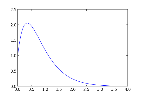
As an example, let γ =1, m = 1, and k = 5. This implies μ =  √19/2. Set the initial conditions so that R = 6 and φ = 1. The solid blue line below is the solution 6 exp(-t/2) cos(t– 1), and the dotted green lines above and below are the exponential envelope 6 exp(-t/2).

And here is a video of the mass-spring-dashpot system in action made using the code discussed here.

Note that the solution is not simply an oscillation at the natural frequency multiplied by an exponential term. The damping changes the frequency of the periodic term, though the change is small when the damping is small.

The factor μ is called the quasi-frequency. Recall from the previous post that the natural frequency, the frequency of the solution with no damping, is denoted ω₀. The quasi-frequency is related to the natural frequency by

μ = √(1 – γ²/4mk) ω₀ ≈ (1 – γ²/8mk) ω₀.

The approximation above holds for small γ since a Taylor expansion shows that √(1 – x) ≈ 1 – x/2 for small x.

This says that the quasi-frequency decreases the natural frequency by a factor of approximately γ²/8mk. So when γ is small there is little change to the natural frequency, but the amount of change grows quadratically as γ increases.

Critical damping

Critical damping occurs when γ² = 4mk. In this case the solution is given by

u(t) = (A + Bt) exp( – γt/2m).

The position of the mass will asymptotically approach 0. Depending on the initial velocity, it will either go monotonically to zero or reach some maximum displacement before it turns around and goes to 0.

For an example, let m = 1 and k = 5 as before. For critical damping, γ must equal √20. Choose initial conditions so that A = 1 and B = 10.

Over-damping

When γ² > 4mk the system is over-damped. When damping is that large, the system does not oscillate at all.

The solution is

u(t) = A exp(r₁ t) + B exp(r₂ t)

where r₁ and r₂ are the two roots of

m x² + γ x + k = 0.

Because γ > 0, both roots are negative and solutions decay exponentially to 0.

Coming up

The next two posts in the series will add a forcing term, i.e. F > 0 in our differential equation. The next post will look at undamped driven vibrations, and the final post will look at damped driven vibrations.