Ramanujan’s nested radical

Posted on 13 September 2013 by John

Ramanujan posed the following puzzle to Journal of Indian Mathematical Society. What is the value of the following?

$\sqrt{1+2\sqrt{1+3 \sqrt{1+4\sqrt{1 + \cdots}}}}$

He waited over six months, and when nobody replied he gave his solution. The result is simply 3.

Now suppose you didn’t know an algebraic proof and wanted to evaluate the expression numerically. The code below will evaluate Ramanujan’s expression down to n levels.

def f(n):
    t = 1.0
    for k in range(n, 1, -1):
        t = sqrt(k*t + 1)
    return t

(The range function above produces the sequence n, n-1, … 2.)

The sequence of f(n) values converges rapidly to 3 as the plot below shows.

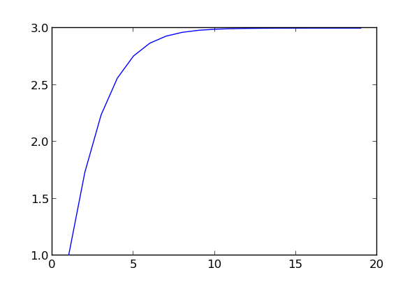
The code above evaluates the expression from the inside out, and so you need to know where you’re going to stop before you start. I don’t see how to write a different algorithm that would let you compute f(n+1) taking advantage of having computed f(n). Do you? Can you think of a way to evaluate f(1), f(2), f(3), … f(N) in less than O(N²) time? Will your algorithm if some or all of the numbers in Ramanujan’s expression change?

Visualizing category concept dependencies

Posted on 10 September 2013 by John

Category theory has a high ratio of definitions to theorems, and it can seem like every definition depends on an infinite regress of definitions. But if you graph the definition dependencies, the graph is wide rather than deep.

I picked out 65 concepts and created a visualization using GraphViz. No definition is more than six degrees away from first principles, and most are closer. The graph is pretty big, so here’s a thumbnail.

The full graph is available here.

It’s possible to define concepts in different ways and obtain a different graph. I used definitions from here.

Here is a list of other math diagrams I’ve created.

Related: Applied category theory

Heidelberg Laureate Forum

Posted on 9 September 2013 by John

I will be going to Germany in a couple weeks to be a blogger for the Heidelberg Laureate Forum. This conference will bring young researchers in math and computer science together with some of the top people in their fields, winners of the Abel Prize, Turing Award, Fields Medal, and Nevanlinna Prize. I’m looking forward to visiting Heidelberg and being part of an incredible conference.

Heidelberg castle photo via Wikipedia

How hospitals make decisions

Posted on 7 September 2013 by John

From operations research professor Michael Carter on The Science of Better:

If I went into a company, a private company, and said “I can save you a million dollars day,” the CEO would implement it tomorrow. If I went into a hospital and said “I can save you a million dollars a day,” they’d they have to think about it, because the CEO would have to convince people this was a good idea. It would have to be good for the doctors, good for the nurses, good for the bean counters, good for the patients, good for patient quality, good for media. … All problems become multi-criteria problems. The good new is that things are so bad in health care we can always do that.

That matches my experience from when I used to work for a hospital.

Carter’s last line may not be clear in the excerpt above. In context, he’s saying that health care is so inefficient that an operations research consultant can always find ways to improve things, even though decisions have to satisfy numerous constituencies.

Nicholas Carr said something similar in his book Does IT Matter? Carr argues for most of the book that although information technology is important, it has become a given, like electricity. Then near the end of his book, he says that because health care IT is so far behind, his remarks don’t apply there.

Homework problems for 2090

Posted on 4 September 2013 by John

In his 1990 article “Has progress in mathematics slowed down?” Paul Halmos mentions two of the longest proofs in mathematics: the Four Color Theorem and the classification of finite simple groups.

The proof of the Four Color Theorem appeared in 1976. The authors manually broke the problem into 1,936 cases which were then verified using a computer. The classification of finite simple groups was the culmination of many journal articles totaling around 10,000 pages.

Halmos believed that these were not “good” proofs. They establish the truth of their claims, but they are so large and tedious that they don’t give much insight into their subjects. He also believed that over time the proofs of both theorems would be simplified.

A hundred years from now both theorems (maps and groups) will be exercises for first-year graduate courses, provable in a couple pages by means of the appropriate concepts, which will be completely familiar by then.

(Emphasis added.)

So where do we stand, 23 years later? The number of special cases required for the Four Color Theorem has been reduced to 633, about one third of the original number. The proof has been verified via the Coq proof assistant software but is still requires a computer. There is an ongoing effort to produce a “second generation” proof of the classification of finite simple groups. This effort is expected to fill around 5,000 pages, half the original count, and also to be easier to read.

Halmos said that over time,

… mathematics shortens proofs, gives insight, and deepens understanding by the discovery of new concepts and by the subsumption of old ones under a suitably general theory that took years, decades, and sometimes centuries of labor to construct.

This has happened for the two theorems under discussion here, but not yet to a very large extent. If we assume the size of the classification of finite simple groups is decreasing exponentially, it will still be 625 pages in the year 2090. But progress in mathematics isn’t so predictable. The proof may hover at 5000 pages for decades, then suddenly collapse to 100 pages after some brilliant breakthrough. A two-page proof by 2090 seems unlikely. I doubt Halmos meant his prediction literally, but it would be interesting to see where things stand by then. (Someone mark your calendar to write a follow-up blog post in 77 years in case I stop blogging before then.)

Naming collections

Posted on 3 September 2013 by John

When you have an array of things, do you name the array with a plural noun because it contains many things, or you name it with a singular noun because each thing it contains is singular? For example, if you have a collection of words, should you name it words or word?

Does it make any difference if you’re using some container other than an array? For example if you have a dictionary (a.k.a. map, hash, associative array, etc.) counting word frequencies, should it be count or counts?

I’ve never had a convention that I consciously follow. But I’ve often stopped to wonder which way I should name things. One approach may look right when I declare a variable and another when I use it.

Damian Conway has a reasonable suggestion in his book Perl Best Practices. (There are many things in that book that are good advice for people who never touch Perl.) He recommends using plural names for most arrays and singular names for dictionaries and arrays used like dictionaries.

Because hash entries are typically accessed individually, it makes sense for the hash itself to be named in the singular. That convention causes the individual accesses to read more naturally in the code. … On the other hand, array values are more often processed collectively … So it makes sense to name them in the plural, after the group of items they store. … If, however, an array is to be used as a random-access look-up table, name it in the singular, using the same conventions as a hash.

A magic square filled with consecutive primes

Posted on 2 September 2013 by John

In 1988 Martin Gardner offered a $100 prize for the first person to produce a magic square filled with consecutive primes. Later that year, Harry Nelson found 22 solutions using a Cray computer.

1,480,028,201	1,480,028,129	1,480,028,183
1,480,028,153	1,480,028,171	1,480,028,189
1,480,028,159	1,480,028,213	1,480,028,141

Gardner said that the square above is “almost certainly the one with the lowest constant possible for such a square.”

It’s easy to verify that the numbers above are consecutive primes. Here’s a little Python code for the job. The function nextprime(x, i) gives the next i primes after x. We call the function with x equal to one less than the smallest entry in the square and it prints out all the entries.

    from sympy import nextprime
    for i in range(1,10):
        print( nextprime(148028128, i) )

If you’re looking for more than a challenge, verify whether Gardner’s assertion was correct that the square above uses the smallest possible set of consecutive primes.

By the way, assuming Harry Nelson’s Cray was the Y-MP model that came out in 1988, here are its specs according to Wikipedia:

The Y-MP could be equipped with two, four or eight vector processors, with two functional units each and a clock cycle time of 6 ns (167 MHz). Peak performance was thus 333 megaflops per processor. Main memory comprised 128, 256 or 512 MB of SRAM.

Related: Magic squares from a knight’s tour and a king’s tour.

The Jericho-Masada approach to mathematics

Posted on 2 September 2013 by John

Pierre Cartier describing Alexander Grothendieck’s approach to mathematics:

Grothendieck’s favorite method is not unlike Joshua’s method for conquering Jericho. The thing was to patiently encircle the solid walls without actually doing anything: at a certain point, the walls fall flat without a fight. This was also the method used by the Romans when they conquered the natural desert fortress Masada, the last stronghold of the Jewish revolt, after spending months patiently building a ramp. Grothendieck was convinced that if one has a sufficiently unifying vision of mathematics, if one can sufficiently penetrate the essence of mathematics and the strategies of its concepts, then particular problems are nothing but a test; they do not need to be solved for their own sake.

Source

Relating Airy and Bessel functions

Posted on 1 September 2013 by John

The Airy functions Ai(x) and Bi(x) are independent solutions to the differential equation

For negative x they act something like sin(x) and cos(x). For positive x they act something like exp(x) and exp(-x). This isn’t surprising if you look at the differential equation. If you replace x with a negative constant, you get sines and cosines, and if you replace it with a positive constant, you get positive and negative exponentials.

The Airy functions can be related to Bessel functions as follows:

$\mathrm{Ai}(x) = \left\{ \begin{array}{ll} \frac{1}{3}\sqrt{\phantom{-}x} \left(I_{-1/3}(\hat{x}) - I_{1/3}(\hat{x})\right) & \mbox{if } x > 0 \\ \\ \frac{1}{3}\sqrt{-x} \left(J_{-1/3}(\hat{x}) + J_{1/3}(\hat{x})\right) & \mbox{if } x < 0 \end{array} \right.$

and

$\mathrm{Bi}(x) = \left\{ \begin{array}{ll} \sqrt{\phantom{-}x/3} \left(I_{-1/3}(\hat{x}) + I_{1/3}(\hat{x})\right) & \mbox{if } x > 0 \\ \\ \sqrt{-x/3} \left(J_{-1/3}(\hat{x}) - J_{1/3}(\hat{x})\right) & \mbox{if } x < 0 \end{array} \right.$

Here J is a “Bessel function of the first kind” and I is a “modified Bessel function of the first kind.” Also

$\hat{x} = \frac{2}{3} \left(\sqrt{|x|}\right)^3$

To verify the equations above, and to show how to compute these functions in Python, here’s some code.

The SciPy function airy computes both functions, and their first derivatives, at once. I assume that’s because it doesn’t take much longer to compute all four functions than to compute one. The code for Ai2 and Bi2 below uses np.where instead of if … else so that it can operate on NumPy vectors all at once. You can plot Ai and Ai2 and see that the two curves lie on top of each other. The same holds for Bi and Bi2.

from scipy.special import airy, jv, iv
from numpy import sqrt, where

def Ai(x):
    (ai, ai_prime, bi, bi_prime) = airy(x)
    return ai

def Bi(x):
    (ai, ai_prime, bi, bi_prime) = airy(x)
    return bi

def Ai2(x):
    third = 1.0/3.0
    hatx = 2*third*(abs(x))**1.5
    return where(x > 0,
        third*sqrt( x)*(iv(-third, hatx) - iv(third, hatx)),
        third*sqrt(-x)*(jv(-third, hatx) + jv(third, hatx)))

def Bi2(x):
    third = 1.0/3.0
    hatx = 2*third*(abs(x))**1.5
    return where(x > 0,
        sqrt( x/3.0)*(iv(-third, hatx) + iv(third, hatx)),
        sqrt(-x/3.0)*(jv(-third, hatx) - jv(third, hatx)))

There is a problem with Ai2 and Bi2: they return nan at 0. A more careful implementation would avoid this problem, but that’s not necessary since these functions are only for illustration. In practice, you’d simply use airy and it does the right thing at 0.

Related links:

Month: September 2013