Create a graph by first making a set of n vertices and then connecting nodes i and j, i > j, with probability p. This is known as the Erdős-Rényi graph Gn,p. Here’s such a graph with n = 100 and p = 0.1.
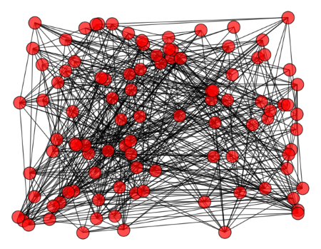
Then the spectrum of the adjacency matrix A of the graph bounces around the spectrum of the expected value of A. This post will illustrate this to give an idea how close the two spectra are.
The adjacency matrix A for our random graph has zeros along the diagonal because the model doesn’t allow loops connecting a vertex with itself. The rest of the entries are 1 with probability p and 0 with probability 1-p. The entries above the diagonal are independent of each other, but the entries below the diagonal are determined by the entries above by symmetry. (An edge between i and j is also an edge between j and i.)
The expected value of A is a matrix with 0’s along the diagonal and p‘s everywhere else. This matrix has one eigenvalue of p(n – 1) and (n – 1) eigenvalues –p. Let’s see how close the spectra of a dozen random graphs come the spectra of the expected adjacency matrix. As above, n = 100 and p = 0.1.
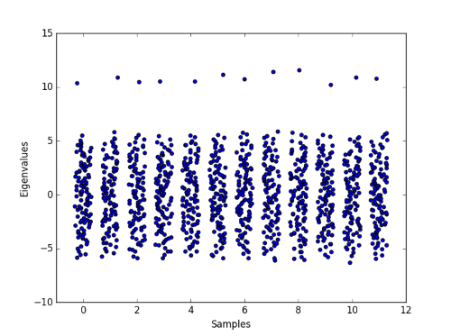
Because the eigenvalues are close together, I jittered each sample horizontally to make the values easier to see. Notice that the largest eigenvalue in each sample is around 10. The expected value is p(n – 1) = 9.9, so the values are close to their expected value.
The other eigenvalues seem to be centered around 0. This is consistent with the expected value of –p = -0.1. The most obvious thing about the smaller eigenvalues is not their mean but their range. How far can might the eigenvalues be from their expected value? Fan Chung and Mary Radcliffe give the following estimate in their paper On the Spectra of General Random Graphs.
For Gn,p, if p > 8 log(√2 n)/9n, then with probability at least 1 – 1/n we have

Here J is the matrix of all 1’s and I is the identity matrix. In our case the theorem says that with probability at least 0.99, we expect the eigenvalues of our random graph to be within 19.903 of their expected value. This is a pessimistic bound since no value is much more than 5 away from its expected value.
Being a novice eigenvalue-er, trying to develop a sense of what the various eigenvalues stand for. Assuming that a ball is being passed along the edges of the graph. Then the high eigenvalue belongs to the eigenvector of stationary distribution of the of the ball. That is, if the ball is with 1/n probability in any of the verticies, then multiplying the state probability vector with the transition probability matrix A, we arrive to p(n-1).
Is there such an intuitive explanation of the other eigenvalues too?
Mark, the A matrix does not conserve the probability densitity to sum up to 1.
So the sum of the rows are not 1.
So it is not a transition matrix, unfortunatelly.
However, its easy to “save” your argument. Just multiply the matrix A by 1/((N-1)*p), it can be forced to be a transition matrix.
BTW it is the special case when p = 1/(N-1).
In this case, the biggest eigenvalue is 1, which is indeed p(N-1), s.
Eiegenvalues tranform linearlly, so the biggest eigenvalue in the original case is indeed p*(N-1).
BTW the eigen-vector is the symmetric solution [1/N,…,1/N], as the transition has also symmetrical, so a symmetric distribution must remain symmetric. :)
For the other eigenvecors, they are not positives (so there are positive and negative elements as well), but there should be some intutition behind the -p eigenvalues too…. i could not find this so far. But there must be some symmetry, so they can be anti-symmetrical solutions, i will think about it…
I think this is somehow intuitive (but works only for the case p=1/(N-1))
But if we can think of transition more generally (the just weights instead of probability distribution)
Thanks for the correction, the transition probability matrix is of course A/(n-1).
I wonder if this (Erdős-Rényi graph) could help to model information spread among traders or institutions.
The transition probability matrix is of course A/((N-1)*p)!
Mark asked what is the intuitin behind -p eigenvalues. I try to answer.
So first, let scale the matrix A to be a transition matrix, so p=1/(N-1).
(We dont loose generality, then we can scale back the result.)
So, the largest eigenvalue is 1, and it corresponds the stacionary distribution.
which is uniform, u=[1/N,1/N,…,1/N].
This come directly from symmetry, and is quite intuitive: if we start a ball from a node, after a very long time the ball will be (almost) eqaull likley at any node.
Now let see an arbitratry distribution vector x, we can decompose it to the uniform (u), and the rest (v).
x = u + v
As sum(x)=1, and sum(u)=1, so sum(v)=0.
The egeinvalues -p means that this deviation decay exponentially, with exponent p, also oscillates. But why the eigenvalue is -p?
Let see what happens with v, is we multiply with A.
Each element will be the sum of the other elements times p, or, the average of the other elements. But the sum is zero, so the sum of the other elements are just the opposite of this elements. And this opposite will be also multiplied by p. So each elements will be just -p times itself. So Av = -p * v.
After k timestep, x_k = u + (-p)^k * v.
with any start configuration, the deviation from the uniform is decrease exponentially , and change sign in each step.
So e.g. if start a ball from node 1, each odd step node1 prob IS smaller then 1/N. Step 1 is zero (devation -1/N).
each even step prob is larger then 1/N. But the difference decays as p over k.
The system has some memory of the initial condition, but this eleminted exponentially.
Some generalization:
* any graph, if all other eigenvalues is smaller then 1 in absolute value, then the distribution will converge to the stacionaire.
* any grah symmetic to permuation will have uniform stacinonaire dist.
* if eigenvalue is -1, then the initial deviation NEVER disapper. This is the case in a cyclic graph with even node!