Solutions to differential equations often satisfy some sort of maximum principle, which can in turn be used to construct upper and lower bounds on solutions.
We illustrate this in one dimension, using a boundary value problem for an ordinary differential equation (ODE).
Maximum principles
If the second derivative of a function is positive over an open interval (a, b), the function cannot have a maximum in that interval. If the function has a maximum over the closed interval [a, b] then it must occur at one of the ends, at a or b.
This can be generalized, for example, to the following maximum principle. Let L be the differential operator
L[u] = u” + g(x)u’ + h(x)
where g and h are bounded functions on some interval [a, b] and h is non-positive. Suppose L[u] ≥ 0 on (a, b). If u has an interior maximum, then u must be constant.
Boundary value problems
Now suppose that we’re interested in the boundary value problem L[u] = f where we specify the values of u at the endpoints a and b, i.e. u(a) = ua and u(b) = ub. We can construct an upper bound on u as follows.
Suppose we find a function z such that L[z] ≤ f and z(a) ≥ ua and z(b) ≥ ub. Then by applying the maximum principle to u – z, we see that u – z must be ≤ 0, and so z is an upper bound for u.
Similarly, suppose we find a function w such that L[w] ≥ f and w(a) ≤ ua and w(b) ≤ ub. Then by applying the maximum principle to w – u, we see that w – u must be ≤ 0, and so w is an lower bound for u.
Note that any functions z and w that satisfy the above requirements give upper and lower bounds, though the bounds may not be very useful. By being clever in our choice of z and w we may be able to get tighter bounds. We might start by choosing polynomials, exponentials, etc. Any functions that are easy to work with and see how good the resulting bounds are.
Tomorrow’s post is similar to this one but looks at bounds for an initial value problem rather than a boundary value problem.
Airy equation example
The following is an elaboration on an example from [1]. Suppose we want to bound solutions to
u”(x) – x u(x) = 0
where u(0) = 0 and u(1) = 1. (This is a well-known equation, but for purposes of illustration we’ll pretend at first that we know nothing about its solutions.)
For our upper bound, we can simply use z(x) = x. We have L[z] ≤ 0 and z satisfies the boundary conditions exactly.
For our lower bound, we use w(x) = x – βx(1 – x). Why? The function z already satisfies the boundary condition. If we add some multiple of x(1 – x) we’ll maintain the boundary condition since x(1 – x) is zero at 0 and 1. The coefficient β gives us some room to maneuver. Turns out L[w] ≥ 0 if β ≥ 1/2. If we choose β = 1/2 we have
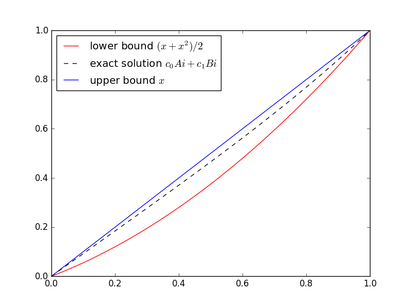
(x + x2)/2 ≤ u(x) ≤ x
In general, you don’t know the function you’re trying to bound. That’s when bounds are most useful. But this is a sort of toy example because we do know the solution. The equation in this example is well known and is called Airy’s equation. The Airy functions Ai and Bi are independent solutions. Here’s a plot of the solution with its upper and lower bounds.

Here’s the Python code I used to solve for the coefficients of Ai and Bi and make the plot.
import numpy as np
from scipy.linalg import solve
from scipy.special import airy
import matplotlib.pyplot as plt

# airy(x) returns (Ai(x), Ai'(x), Bi(x), Bi'(x))
def Ai(x):
    return airy(x)[0]

def Bi(x):
    return airy(x)[2]

M = np.matrix([[Ai(0), Bi(0)], [Ai(1), Bi(1)]])
c = solve(M, [0, 1])

t = np.linspace(0, 1, 100)
plt.plot(t, (t + t**2)/2, 'r-', t, c[0]*Ai(t) + c[1]*Bi(t), 'k--', t, t, 'b-',)
plt.legend(["lower bound $(x + x^2)/2$",
    "exact solution $c_0Ai + c_1Bi$",
    "upper bound $x$"], loc="upper left")
plt.show()
SciPy’s function airy has an optimization that we waste here. The function computes Ai and Bi and their first derivatives all at the same time. We could take advantage of that to remove some redundant computations, but that would make the code harder to read. We chose instead to wait an extra nanosecond for the plot.
Help with differential equations
* * *
[1] Murray Protter and Hans Weinberger. Maximum Principles in Differential Equations.

Comments are closed.