Surprise index
Warren Weaver [1] introduced what he called the surprise index to quantify how surprising an event is. At first it might seem that the probability of an event is enough for this purpose: the lower the probability of an event, the more surprise when it occurs. But Weaver’s notion is more subtle than this.
Let X be a discrete random variable taking non-negative integer values such that

Then the surprise index of the ith event is defined as

Note that if X takes on values 0, 1, 2, … N−1 all with equal probability 1/N, then Si = 1, independent of N. If N is very large, each outcome is rare but not surprising: because all events are equally rare, no specific event is surprising.
Now let X be the number of legs a human selected at random has. Then p2 ≈ 1, and so the numerator in the definition of Si is approximately 1 and S2 is approximately 1, but Si is large for any value of i ≠ 2.
The hard part of calculating the surprise index is computing the sum in the numerator. This is the same calculation that occurs in many contexts: Friedman’s index of coincidence, collision entropy in physics, Renyi entropy in information theory, etc.
Poisson surprise index
Weaver comments that he tried calculating his surprise index for Poisson and binomial random variables and had to admit defeat. As he colorfully says in a footnote:
I have spent a few hours trying to discover that someone else had summed these series and spent substantially more trying to do it myself; I can only report failure, and a conviction that it is a dreadfully sticky mess.
A few years later, however, R. M. Redheffer [2] was able to solve the Poisson case. His derivation is extremely terse. Redheffer starts with the generating function for the Poisson

and then says
Let x = eiθ; then e−iθ; multiply; integrate from 0 to 2π and simplify slightly to obtain

The integral on the right is recognized as the zero-order Bessel function …
Redheffer then “recognizes” an expression involving a Bessel function. Redheffer acknowledges in a footnote at a colleague M. V. Cerrillo was responsible for recognizing the Bessel function.
It is surprising that the problem Weaver describes as a “dreadfully sticky mess” has a simple solution. It is also surprising that a Bessel function would pop up in this context. Bessel functions arise frequently in solving differential equations but not that often in probability and statistics.
Unpacking Redheffer’s derivation
When Redheffer says “Let x = eiθ; then e−iθ; multiply; integrate from 0 to 2π” he means that we should evaluate both sides of the equation for the Poisson generating function equation at these two values of x, multiply the results, and average the both sides over the interval [0, 2π].
On the right hand side this means calculating

This reduces to

because

i.e. the integral evaluates to 1 when m = n but otherwise equals zero.
On the left hand side we have

Cerrillo’s contribution was to recognize the integral as the Bessel function J0 evaluated at -2iλ or equivalently the modified Bessel function I0 evaluated at -2λ. This follows directly from equations 9.1.18 and 9.6.16 in Abramowitz and Stegun.
Putting it all together we have

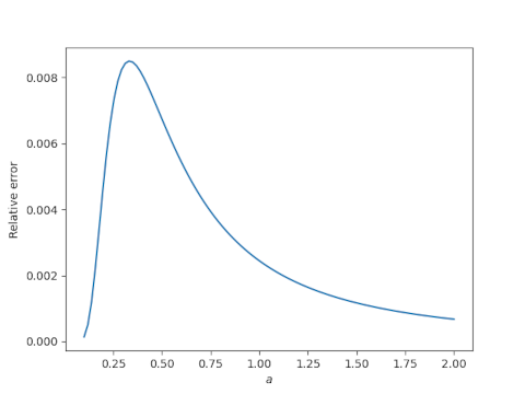
Using the asymptotic properties of I0 Redheffer notes that for large values of λ,

[1] Warren Weaver, “Probability, rarity, interest, and surprise,” The Scientific Monthly, Vol 67 (1948), p. 390.
[2] R. M. Redheffer. A Note on the Surprise Index. The Annals of Mathematical Statistics, Mar., 1951, Vol. 22, No. 1 pp. 128ndash;130.