Error in the normal approximation to the Poisson distribution

If X ~ Poisson(λ) with λ “large” then X is well approximated by a normal distribution. This page looks at this approximation in detail. For example, how large does λ have to be? For a fixed value of λ, how does the error vary? Where is it best and worst?

Central Limit Theorem

First we show why there is a normal approximation to the Poisson. If X₁ and X₂ are independent Poisson random variables with means λ₁ and λ₂ then X₁ + X₂ has a Poisson distribution with mean λ₁ + λ₂. This means that a Poisson random variable X with mean λ has the same distribution as the sum of N independent Poisson random variables X_i with mean λ/N. We can apply the Central Limit Theorem to this sum to show that X has approximately the same distribution as a normal random variable Y with mean λ and variance λ, the same mean and variance as X.

General bound on error

To measure the error in the normal approximation, let F_X be the cumulative distribution function (CDF) of X and F_Y be the CDF of Y, the normal approximation to X. We can apply the Berry-Esséen theorem to ∑X_i to show that |F_X(x) – F_Y(x)| is bounded by C/√λ for all x where C is some constant less than 0.7164. (This summary leaves out some subtle details.)

The bound from the Berry-Esséen theorem is pessimistic, but it shows right away that the error decreases as λ increases. The bound over-estimates the error for two reasons. First, it’s based on a general theorem that doesn’t use any special knowledge of the Poisson distribution other than its second and third moments. Second, it doesn’t take into account a continuity correction that improves the approximation.

Example

The following plot shows the probability mass function (PMF) for a Poisson distribution with λ = 10.

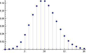
This shows there’s good reason to believe the Poisson and normal distributions are connected.

Error in approximating the CDF

Next we want to look at the error in the normal approximation to the Poisson distribution. Let X be a Poisson random variable with mean λ and let Y be a normal random variable with mean and variance λ. Denote the PMFs of X and Y by f_X and f_Y and denote the CDFs of X and Y by F_X and F_Y.

First we look at F_X – F_Y and we show what an improvement the continuity correction makes. Then we look at the error in approximating the probability of individual points by looking at f_X and f_Y.

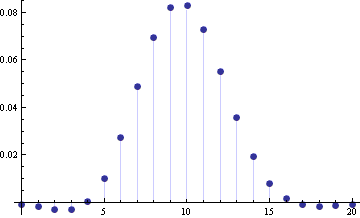
The following graph shows F_X(n) – F_Y(n) for n = 0, 1, 2, …, 20.

Next we look at F_X(n) – F_Y(n + ½). The reason for adding this extra ½ is the continuity correction we will discuss below.

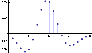
The Berry–Esséen theorem gives an upper bound of 0.7164/√10 = 0.2265 for the approximation error. The maximum error without the continuity correction is 0.083. With the continuity correction, the maximum error goes down to 0.021. So in this case the actual error is about three times smaller than the theoretical bound, and the continuity correction reduces the error by another factor of 4. These ratios are typical as λ varies.

In the previous example, the maximum error occurred at n = λ without the error continuity correction and at λ-1 with the continuity correction. This appears to be true in general; I’ve numerically verified that it is true for integer values of λ ≤ 100.

Error in approximating the PMF

Now we turn our attention to approximating f_X(n) by the integral

which approximates P(X = n) by P(n-½ < Y < n+½). Adding up the approximations for several values of n explains the extra factor of ½ in the continuity correction in the CDF approximation.

While the error in approximating the CDF is has a maximum value near λ, the error in approximating the PMF has a local minimum near λ. However, the error grows quickly on either side of λ. The following graph plots f_X(n) minus its approximation for λ = 20.

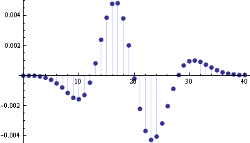
The absolute value of the error is smallest in the tails. However, the relative error in the approximation is smallest near the mean and is larger in the tails. The following graph gives the signed relative error.

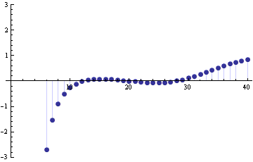
The graph is truncated because the relative errors on the far left are enormous. The relative error at 0 is -2000 and the relative error at 1 is -250.

Other normal approximations

There are other less direct ways to form normal approximations to the Poisson distribution function. See notes on the Wilson-Hilferty normal approximation. This method is often far more accurate than the approximation above.

See also notes on the normal approximation to the beta, binomial, gamma, and student-t distributions.