Fluctuation strength is similar to roughness, though at much lower modulation frequencies. Fluctuation strength is measured in vacils (from vacilare in Latin or vacillate in English). Police sirens are a good example of sounds with high fluctuation strength.
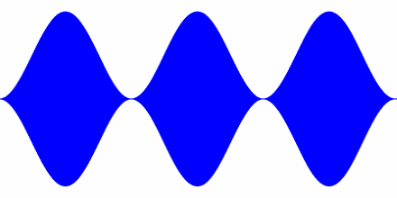
Fluctuation strength reaches its maximum at a modulation frequency of around 4 Hz. For much higher modulation frequencies, one perceives roughness rather than fluctuation. The reference value for one vacil is a 1 kHz tone, fully modulated at 4 Hz, at a sound pressure level of 60 decibels. In other words
(1 + sin(8πt)) sin(2000πt)
where t is time in seconds.
Since the carrier frequency is 250 times greater than the modulation frequency, you can’t see both in the same graph. In this plot, the carrier is solid blue compared to the modulation.
Here’s what the reference for one vacil would sound like:
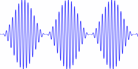
Acoustic roughness is measured in aspers (from the Latin word for rough). An asper is the roughness of a 1 kHz tone, at 60 dB, 100% modulated at 70 Hz. That is, the signal
(1 + sin(140πt)) sin(2000πt)
where t is time in seconds.
Here’s what that sounds like (if you play this at 60 dB, about the loudness of a typical conversation at one meter):
And here’s the Python code that made the file:
    from scipy.io.wavfile import write
    from numpy import arange, pi, sin, int16

    def f(t, f_c, f_m):
        # t    = time
        # f_c  = carrier frequency
        # f_m  = modulation frequency
        return (1 + sin(2*pi*f_m*t))*sin(2*f_c*pi*t)

    def to_integer(signal):
        # Take samples in [-1, 1] and scale to 16-bit integers,
        # values between -2^15 and 2^15 - 1.
        return int16(signal*(2**15 - 1))

    N = 48000 # samples per second
    x = arange(3*N) # three seconds of audio

    # 1 asper corresponds to a 1 kHz tone, 100% modulated at 70 Hz, at 60 dB
    data = f(x/N, 1000, 70)
    write("one_asper.wav", N, to_integer(data))
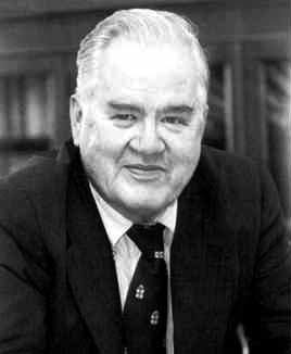
John Tukey coined many terms that have passed into common use, such as bit (a shortening of binary digit) and software. Other terms he coined are well known within their niche: boxplot, ANOVA, rootogram, etc. Some of his terms, such as jackknife and vacuum cleaner, were not new words per se but common words he gave a technical meaning to.
Cepstrum is an anagram of spectrum. It involves an unusual use of power spectra, and is roughly analogous to making anagrams of a word. A related term, one we will get to shortly, is quefrency, an anagram of frequency. Some people pronounce the ‘c’ in cepstrum hard (like ‘k’) and some pronounce it soft (like ‘s’).
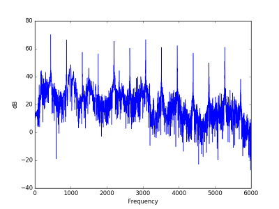
Let’s go back to an example from my post on guitar distortion. Here’s a note played with a fairly large amount of distortion:
And here is its power spectrum:
There’s a lot going on in the spectrum, but the peaks are very regularly spaced. As I mentioned in the post on the sound of a leaf blower, this is the fingerprint of a sound with a definite pitch. Spikes in the spectrum alone don’t indicate a definite pitch if they are irregularly spaced.
The peaks are fairly periodic. How to you find periodic patterns in a signal? Fourier transform! But if you simply take the Fourier transform of a Fourier transform, you essentially get the original signal back. The key to the cepstrum is to do something else between the two Fourier transforms.
The cepstrum starts by taking the Fourier transform, then the magnitude, then the logarithm, and then the inverse Fourier transform.
When we take the magnitude, we throw away phase information, which we don’t need in this context. Taking the log of the magnitude is essentially what you do when you compute sound pressure level. Some define the cepstrum using the magnitude of the Fourier transform and some the magnitude squared. Squaring only introduces a multiple of 2 once we take logs, so it doesn’t effect the location of peaks, only their amplitude.
Taking the logarithm compresses the peaks, bringing them all into roughly the same range, making the sequence of peaks roughly periodic.
When we take the inverse Fourier transform, we now have something like a frequency, but inverted. This is what Tukey called quefrency.
Looking at the guitar power spectrum above, we see a sequence of peaks spaced 440 Hz apart. When we take the inverse Fourier transform of this, we’re looking at a sort of frequency of a frequency, what Tukey calls quefrency. The quefrency scale is inverted: sounds with a high frequency fundamental have overtones that are far apart on the frequency domain, so the sequence of the overtone peaks has low frequency.
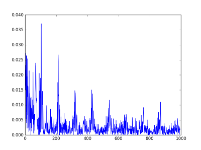
Here’s the plot of the cepstrum for the guitar sample.
There’s a big peak at 109 on the quefrency scale. The audio clip was recorded at 48000 samples per second, so the 109 on the quefrency scale corresponds to a frequency of 48000/109 = 440 Hz. The second peak is at quefrency 215, which corresponds to 48000/215 = 223 Hz. The second peak corresponds to the perceived pitch of the note, A3, and the first peak corresponds to its first harmonic, A4. (Remember the quefrency scale is inverted relative to the frequency scale.)
I cheated a little bit in the plot above. The very highest peaks are at 0. They are so large that they make it hard to see the peaks we’re most interested in. These low quefrency peaks correspond to very high frequency noise, near the edge of the audible spectrum or beyond.
This afternoon I was working on a project involving tonal prominence. I stepped away from the computer to think and was interrupted by the sound of a leaf blower. I was annoyed for a second, then I thought “Hey, a leaf blower!” and went out to record it. A leaf blower is a great example of a broad spectrum noise with strong tonal components. Lawn maintenance men think you’re kinda crazy when you say you want to record the noise of their equipment.
The tuner app on my phone identified the sound as an A3, the A below middle C, or 220 Hz. Apparently leaf blowers are tenors.
Here’s a short audio clip:
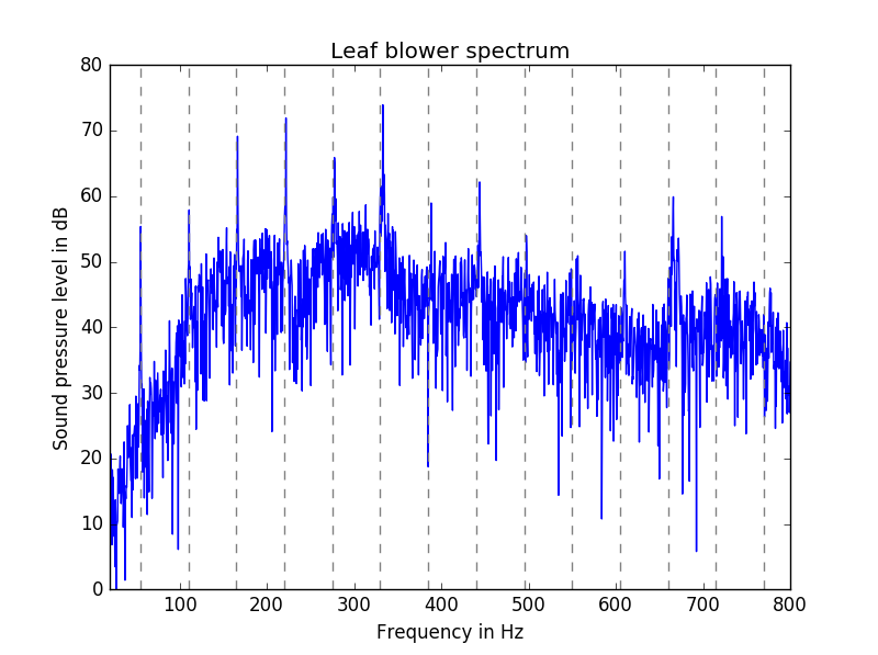
And here’s what the spectrum looks like. The dashed grey vertical lines are at multiples of 55 Hz.
The peaks are perfectly spaced at multiples of the fundamental frequency of 55 Hz, A1 in scientific pitch notation. This even spacing of peaks is the fingerprint of a definite tone. There’s also a lot of random fluctuation between peaks. That’s the finger print of noise. So together we hear a pitch and noise.
When using the tone-to-noise ratio algorithm from the ECMA-74, only the spike at 110 Hz is prominent. A limitation of that approach is that it only considers single tones, not how well multiple tones line up in a harmonic sequence.
This post looks at loudness and sharpness, two important psychoacoustic metrics. Because they have to do with human perception, these factors are by definition subjective. And yet they’re not entirely subjective. People tend to agree on when, for example, one sound is twice as loud as another, or when one sound is sharper than another.
Loudness
Loudness is the psychological counterpart to sound pressure level. Sound pressure level is a physical quantity, but loudness is a psychoacoustic quantity. The former has to do with how a microphone perceives sound, the latter how a human perceives sound. Sound pressure level in dB and loudness in phon are roughly the same for a pure tone of 1 kHz. But loudness depends on the power spectrum of a sound and not just it’s sound pressure level. For example, if a sound’s frequency is too high or too low to hear, it’s not loud at all! See my previous post on loudness for more background.
Let’s take the four guitar sounds from the previous post and scale them so that each has a sound pressure level of 65 dB, about the sound level of an office conversation, then rescale so the sound pressure is 90 dB, fairly loud though not as loud as a rock concert. [Because sound perception is so nonlinear, amplifying a sound does not increase the loudness or sharpness of every component equally.]
While all four sounds have the same sound pressure level, the undistorted sounds have the lowest loudness. The distorted sounds are louder, especially the single note. Increasing the sound pressure level from 65 dB to 90 dB increases the loudness of each sound by roughly the same amount. This will not be true of sharpness.
Sharpness
Sharpness is related how much a sound’s spectrum is in the high end. You can compute sharpness as a particular weighted sum of the specific loudness levels in various bands, typically 1/3-octave bands. This weight function that increases rapidly toward the highest frequency bands. For more details, see Psychoacoustics: Facts and Models.
The table below gives sharpness, measured in acum, for the four guitar sounds at 65 dB and 90 dB.
Although a clean chord sounds a little louder than a single note, the former is a little sharper. Distortion increases sharpness as it does loudness. The single note with distortion is a little louder than the other sounds, but much sharper than the others.
Notice that increasing the sound pressure level increases the sharpness of the sounds by different amounts. The sharpness of the last sound hardly changes.
The other day I asked on Google+ if someone could make an audio clip for me and Dave Jacoby graciously volunteered. I wanted a simple chord on an electric guitar played with varying levels of distortion. Dave describes the process of making the recording as
Let’s look at the Fourier spectrum at four places in the recording: single note and chord, clean and distorted. These are a 0:02, 0:08, 0:39, and 0:43.
Power spectra
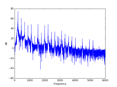
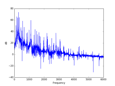
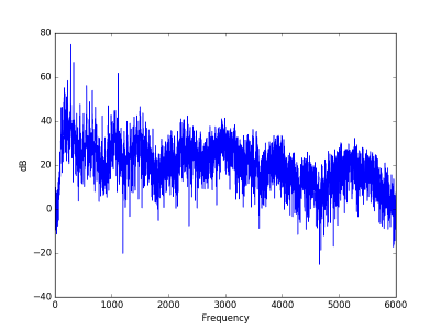
The first note, without distortion, has most of its spectrum concentrated at 220 Hz, the A below middle C.
The same note with distortion has a power spectrum that decays much slow, i.e. the sound has more high frequency components.
Here’s the A major chord without distortion. Note that since the threshold of hearing is around 20 dB, most of the noise components are inaudible.
Here’s the same chord with distortion. Notice there’s much more noise in the audible range.
Update: See the next post an analysis of the loudness and sharpness of the audio samples in this post.
White noise has a flat power spectrum. So a reasonable way to measure how close a sound is to being pure noise is to measure how flat its spectrum is.
Spectral flatness is defined as the ratio of the geometric mean to the arithmetic mean of a power spectrum.
The arithmetic mean of a sequence of n items is what you usually think of as a mean or average: add up all the items and divide by n.
The geometric mean of a sequence of n items is the nth root of their product. You could calculate this by taking the arithmetic mean of the logarithms of the items, then taking the exponential of the result. What if some items are negative? Since the power spectrum is the squared absolute value of the FFT, it can’t be negative.
So why should the ratio of the geometric mean to the arithmetic mean measure flatness? And why pure tones have “unflat” power spectra?
If a power spectrum were perfectly flat, i.e. constant, then its arithmetic and geometric means would be equal, so their ratio would be 1. Could the ratio ever be more than 1? No, because the geometric mean is always less than or equal to the arithmetic mean, with equality happening only for constant sequences.
In the continuous realm, the Fourier transform of a sine wave is a pair of delta functions. In the discrete realm, the FFT will be large at two points and small everywhere else. Why should a concentrated function have a small flatness score? If one or two of the components are 1’s and the rest are zeros, the geometric mean is zero. So the ratio of geometric and arithmetic means is zero. If you replace the zero entries with some small ε and take the limit as ε goes to zero, you get 0 flatness as well.
Sometimes flatness is measured on a logarithmic scale, so instead of running from 0 to 1, it would run from -∞ to 0.
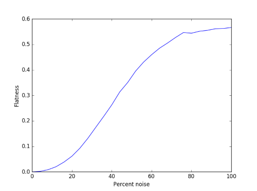
Let’s compute the flatness of some examples. We’ll take a mixture of a 440 Hz sine wave and Gaussian white noise with varying proportions, from pure sine wave to pure noise. Here’s what the flatness looks like as a function of the proportions.
The curve is fairly smooth, though there’s some simulation noise at the right end. This is because we’re working with finite samples.
Here’s what a couple of these signals would sound like. First 30% noise and 70% sine wave:
Why does the flatness of white noise max out somewhere between 0.5 and 0.6 rather than 1? White noise only has a flat spectrum in expectation. The expected value of the power spectrum at every frequency is the same, but that won’t be true of any particular sample.
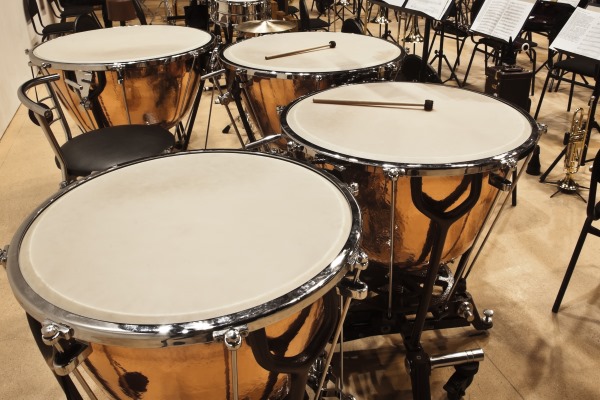
Kettledrums (a.k.a. tympani) produce a definite pitch, but in theory they should not. At least the simplest mathematical model of a kettledrum would not have a definite pitch. Of course there are more accurate theories that align with reality.
Unlike many things that work in theory but not in practice, kettledrums work in practice but not in theory.
A musical sound has a definite pitch when the first several Fourier components are small integer multiples of the lowest component, the fundamental. A pitch we hear at 100 Hz would have a first overtone at 200 Hz, the second at 300 Hz, etc. It’s the relative strengths of these components give each instrument its characteristic sound.
An ideal string would make a definite pitch when you pluck it. The features of a real string discarded for the theoretical simplicity, such as stiffness, don’t make a huge difference to the tonality of the string.
An ideal circular membrane would vibrate at frequencies that are much closer together than consecutive integer multiples of the fundamental. The first few frequencies would be at 1.594, 2.136, 2.296, 2.653, and 2.918 times the fundamental. Here’s what that would sound like:
I chose amplitudes of 1, 1/2, 1/3, 1/4, 1/5, and 1/6. This was somewhat arbitrary, but not unrealistic. Including more than the first six Fourier components would make the sound even more muddled.
By comparison, here’s what it would sound like with the components at 2x up to 6x the fundamental, using the same amplitudes.
This isn’t an accurate simulation of tympani sounds, just something simple but more realistic than the vibrations of an idea membrane.
The real world complications of a kettledrum spread out its Fourier components to make it have a more definite pitch. These include the weight of air on top of the drum, the stiffness of the drum head, the air trapped in the body of the drum, etc.
If you’d like to read more about how kettle drums work, you might start with The Physics of Kettledrums by Thomas Rossing in Scientific American, November 1982.