A general theory of sub-things

When I took my first abstract algebra course, we had a homework question about subgroups. Someone in the class whined that the professor hadn’t told us yet what a subgroup was. My immediate thought was “I bet you could guess. Sub things are all the same. A sub-X is an X contained inside another X. Subset, subspace, subgroup, … They’re all the same.”

My initial reaction was right in that all sub-things are analogous. A subspace is a subset of a vector space that is a vector space in its own right, etc. But there are some hairs that are occasionally worth splitting.

If A is a sub-thing of a thing B, and a is an element of A, sometimes it’s useful to distinguish whether we’re thinking of a as an element of A or whether we’re thinking of a as an element of B. For example, the real numbers are contained in the complex numbers, and when we say -3 has no square root, we implicitly mean -3 as a real number. But if we speak of -3 in complex analysis, say as the location of a pole, we’re thinking of -3 as a complex number, a particular location in the complex plane.

This may all seem pedantic, and it may be, depending on context. But in complicated situations, it can help to make fine distinctions explicit. Novices are unaware of fine distinctions, and sophomores love to point them out, but experts know how to adjust the level of rigor to the appropriate level for a given discussion.

If we want a general theory of sub-things that spans multiple areas of math, we have to use category theory. That’s what category theory is for, codifying patterns that occur across various contexts.

But it seems we’re blocked from the beginning since objects in category theory are black boxes. You cannot speak of parts of an object, so you can’t speak of a subgroup as being a group whose elements belong to another group. You can’t speak of elements at all using the language of category theory.

The only tool at your disposal in category theory is functions. Or to be more precise, morphisms, things that act like functions but might not actually be functions.

What kind of function acts like a subset? Inclusion maps. If A is a subset of B, then there’s a function mapping A into B that sends every point to itself. Going back to the discussion above, an inclusion map is a function that takes a as a member of A to a as a member of B.

Inclusion maps are one-to-one (injective) and so maybe we could use one-to-one functions as our analog of sub-objects.

But saying a function is one-to-one requires looking inside an object and speaking of elements, and that’s not allowed in category theory. And besides, morphisms might not be functions. However, we can say what it means for a morphism to act like a one-to-one function. The categorical counterpart to an injective function is a monomorphism, sometimes just shortened to a “mono.” A subobject of a an object B is a an object A along with a monomorphism from A to B. [1]

By moving from injective functions to monomorphisms we’ve gained something and we’ve lost something.

We’ve gained the notion of preserving structure. For example, a subspace of a vector space isn’t just any subset of a vector space, it’s a linear subspace. In the context of linear algebra we could identify a linear subspace with an injective linear map. When morphisms are functions, they’re not arbitrary functions, but structure-preserving functions, such as linear transformations on linear spaces and continuous functions on topological spaces.

But when we move from subsets to monomorphisms we lose some specificity. If we have a monomorphism from A into B, the object A is only unique up to isomorphism. Everything in category theory is only determined up to isomorphism.

In one way this may be no loss. When we say, for example, that one group is a subgroup of another, maybe all we care about is the structure of the subgroup itself and we don’t care to distinguish isomorphic versions of the subgroup.

But if we’re talking about a manifold M being a submanifold N, we may care which submanifold it is. For example, a circle can be embedded in a torus (doughnut), and it may matter a great deal how we embed it.

If all subobjects are isomorphic, how can we tell them apart? That’s where subobject classifiers come in, a topic I may write about in the future.

More category theory posts

[1] For more on subobjects, see Robert Goldblatt’s book Topoi: The Categorical Analysis of Logic.

One diagram, two completely different meanings

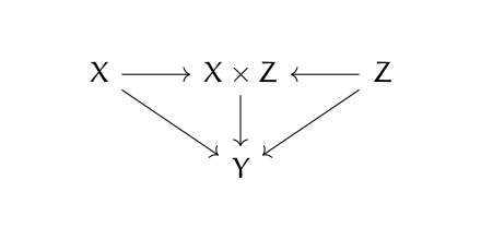
I was thumbing through a new book on causal inference, The Effect by Nick Huntington-Klein, and the following diagram caught my eye.

Then it made my head hurt. It looks like a category theory diagram. What’s that doing in a book on causal inference? And if it is a category theory diagram, something’s wrong. Either there’s a typo or the arrows are backward.

The diagram above is a valid commutative diagram, but for a coproduct rather than a product. That is, X × Z should be labeled X ⨿ Z. (For more on that, see my post on categorical products, and reverse all the arrows in your mind.)

But there’s no category theory going on here. This is an influence diagram. It says that X and Z influence Y directly (indicated by the diagonal arrows), but they also determine the product X × Z (the ordinary product of two numbers, no fancy category stuff) and this product in turn also influences Y.

Related posts

Four, five, and nine lemmas

This post is similar in spirit to the previous post: reducing mathematical theorems to moves in a board game by looking at things from a ridiculously high level.

The theorems we’ll be looking at are known as the four lemma, the five lemma, and the nine lemma. The nine lemma is also known as the 3×3 lemma.

All the lemmas start with a commutative diagram. A diagram is commutative if any two ways of getting from one place to another are equal. If the arrows represent functions, then the diagram implies certain compositions of functions are equal.

Given hypotheses about most of the arrows in a diagram, the theorems conclude something about the rest of the arrows. This general category of theorems is known as diagram chasing. The proofs are tedious but shallow. If a theorem in topology, for example, were formulated as a diagram chase, someone with no intuition for topology could prove the theorem by applying the rules of a simple game.

The meaning of the dots and arrows isn’t important for this post, but you could think of the dots in the diagram as groups and the arrows as homomorphisms between groups. More generally you could think of the dots as objects in an Abelian category and the arrows as morphisms between objects.

The four lemma

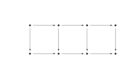
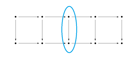
The four lemma starts with a commutative diagram of the following shape.

It’s called the four lemma because there are four dots across each row.

There are two versions of the four lemma. Both make assumptions about the rows and three out of the four columns and conclude something about the fourth column.

In the first part of the lemma, we have hypotheses about the two rows, and hypotheses about the first, third, and fourth vertical arrows. The conclusion is something about the second vertical arrow.

The second part of the lemma is very similar, but has hypotheses about the first, second, and fourth vertical arrows and concludes something about the third arrow.

Five lemma

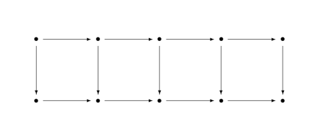
The five lemma starts with a commutative diagram with five objects across the top and bottom rows.

Given assumptions about every arrow except the vertical arrow in the middle, the theorem concludes something about the middle arrow.

Nine lemma

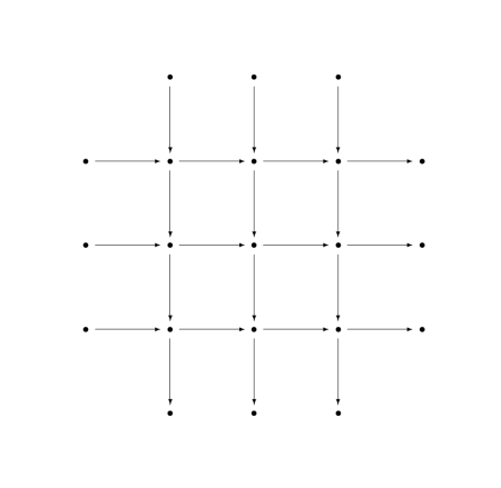
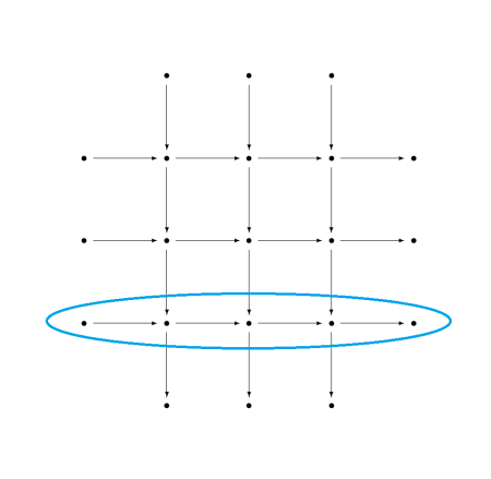
The nine lemma, a.k.a. the 3×3 lemma, starts with a commutative diagram of the following shape.

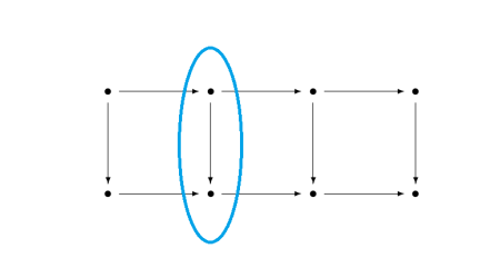
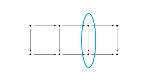
It’s called the nine lemma because the attention is focused on the nine dots, the 3×3 grid of dots in the middle. All the objects around the perimeter, those outside the 3×3 grid, are 0.

There are three parts to the nine lemma. Each has hypotheses about all the columns and two of the rows, and concludes something about the row that was left out. So, for example, one part of the theorem has hypotheses about the three columns and the first two rows and concludes something about the last row.

Missing details

Here I zoom in from 100,000 feet to 10,000 feet, giving some of the missing details but not all. For full details, you could look up the theorems on Wikipedia or on nLab.

As promised at the beginning, this was a ridiculously high-level view of these theorems. The purpose was to point out the core of each theorem and making it possible to compare the three theorems at the highest level.

When I said a theorem makes a hypothesis about a row or a column, the hypothesis is that the row forms an exact sequence. The conclusions in the nine lemma are that a row is an exact sequence.

When I alluded to hypotheses about vertical arrows, these hypotheses are essentially saying that a function is one-to-one (injective), onto (surjective), or one-to-one and onto (bijective). More precisely, they are assumptions that a morphism is mono, epi, or iso. More on this terminology here. The conclusion of the four lemma is that an arrow is either epi or mono. The conclusion of the five lemma is that an arrow is iso.

Related posts

Broadcasting and functors

In my previous post, I looked at the map Δ that takes a column vector to a diagonal matrix. I even drew a commutative diagram, which foreshadows a little category theory.

Suppose you have a function f of a real or complex variable. To an R programmer, if x is a vector, it’s obvious that f(x) means to apply f to every component of a vector. Python (NumPy) works the same way, and calls this broadcasting. To a mathematician, this looks odd. What does the logarithm of a vector, for example, even mean?

As in the previous post, we can use Δ to formalize things. We said that Δ has some nice properties, and in fact we will show it is a functor.

To have a functor, we have to have categories. (Historically, functors came first; categories were defined in order to define functors.) We will define C to be the category of column vectors and M the category of square matrices as before. Or rather, we should say the objects of C are column vectors and the objects of M are square matrices.

Categories need morphisms, functions between objects [1]. We define the morphisms on C to be analytic functions applied componentwise. So, for example, if

z = [1, 2, -3],

then

tan(z) = [tan(1), tan(2), tan(-3)].

The morphisms on M will be analytic functions on square matrices, not applied componentwise but applied by power series. That is, given an analytic function f, we define f of a square matrix X as the result of sticking the matrix X into the power series for f. For an example, see What is the cosine of a matrix?

We said that Δ is a functor. It takes column vectors and turns them into square matrices by putting their contents along the diagonal of a matrix. We gave the example in the previous post that [4, i, π] would be mapped to the matrix with these elements on the diagonal, i.e.

\Delta: \begin{pmatrix} 4 \\ i \\ \pi \end{pmatrix} \mapsto \begin{pmatrix} 4 & 0 & 0\\ 0 & i & 0 \\ 0 & 0 & \pi \end{pmatrix}

That says what Δ does on objects, but what does it do on morphisms? It takes an analytic function that was applied componentwise to column vectors, and turns it into a function that is applied via its power series to square matrices. That is, starting with a function

f(z) = \sum_{n=0}^\infty a_nz^n

we define the morphism f on C by

f : \begin{pmatrix} z_1 \\ z_2 \\ \vdots \\ z_n \end{pmatrix} \mapsto \begin{pmatrix} f(z_1) \\ f(z_2) \\ \vdots \\ f(z_n) \end{pmatrix}

and the morphism Δ f on M by

\Delta f : Z \mapsto \sum_{n=0}^\infty a_n Z^n

where Z is a square matrix.

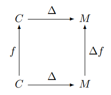
We can apply f to a column vector, and then apply Δ to turn the resulting vector into a diagonal matrix, or we could apply Δ to turn the vector into a diagonal matrix first, and then apply f (technically,  Δf). That is, the follow diagram commutes:

\begin{diagram}   C & \rTo^{\Delta} & M \\   \uTo^{f} & & \uTo_{\Delta f} \\   C & \rTo^{\Delta} & M  \end{diagram}

Python example

Applying an analytic function to a diagonal matrix gives the same result as simply applying the function to the elements of the diagonal. But for more general square matrices, this is not the case. We will illustrate this with some Python code.

    import numpy as np
    from scipy.linalg import funm

    d = np.array([1, 2])
    D = np.diag(d)
    M = np.array([[1, np.pi], [2, 0]])

Now let’s look at some output.

    >>> np.sin(d)                     
    array([0.84147098, 0.90929743])   

    >>> np.sin(D)                     
    array([[0.84147098, 0.        ],  
           [0.        , 0.90929743]]) 

    >>> funm(D, np.sin)               
    array([[0.84147098, 0.        ],  
           [0.        , 0.90929743]]) 

So if we take the sine of d and turn the result into a matrix, we get the same thing as if we turn d into a matrix D and then take the sine of D, either componentwise or as an analytic function (with funm, function of a matrix).

Now let’s look at a general, non-diagonal matrix.

    >>> np.sin(M)
    array([[0.84147099, 0],
       [0.90929743, 0]])

    >>> funm(D, np.sin)
    array([[0.84147098, 0.        ],
           [0.        , 0.90929743]])

Note that the elements in the bottom row are in opposite positions in the two examples.

[1] OK, morphisms are not necessarily functions, but in practice they usually are.

Drawing commutative diagrams with Quiver

I recently discovered quiver, a tool for drawing commutative diagrams. It looks like a nice tool for drawing diagrams more generally, but it’s designed particularly to include the features you need when drawing the kinds of diagrams that are ubiquitous in category theory.

You can draw diagrams using the online app and export the result to LaTeX (tikz).

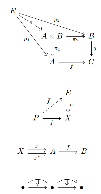
Here are some examples.

quiver diagrams

The app is mostly easy to figure out. The object and arrow labels are specified using LaTeX.

Quiver lets you position labels on either side of an arrow, or even inside the arrow as in the e in the first diagram above.

You can change the arrow and arrowhead styles, as in the second example.

It took me a little while to figure out how to have two arrows with the same destination and source, as in the third example. You use the “offset” setting to move arrows up or down do that they’re not on top of each other. And by default, the software helpfully assumes that if you want to move one arrow up a bit from center, you probably want to move the other one down from center by the same amount.

You can use the “curve” setting to draw arrows as in the final example. You can also draw arrows between arrows, as is common when working with 2-categories.

More category theory posts

Category theory for programmers made easier

I imagine most programmers who develop an interest in category theory do so after hearing about monads. They ask someone what a monad is, and they’re told that if they really want to know, they need to learn category theory.

Unfortunately, there are couple unnecessary difficulties anyone wanting to understand monads etc. is likely to face immediately. One is some deep set theory.

“A category is a collection of objects …”

“You mean like a set?”

“Ah, well, no. You see, Bertrand Russell showed that …”

There are reasons for such logical niceties, but they don’t matter to someone who wants to understand programming patterns.

Another complication is morphisms.

“As I was saying, a category is a collection of objects and morphisms between objects …”

“You mean like functions?”

“Well, they might be functions, but more generally …”

Yes, Virginia, morphisms are functions. It’s true that they might not always be functions, but they will be functions in every example you care about, at least for now.

Category theory is a framework for describing patterns in function composition, and so that’s why things like monads find their ultimate home in category theory. But doing category theory rigorously requires some setup that people eager to get into applications don’t have to be concerned with.

Patrick Honner posted on Twitter recently that his 8-year-old child asked him what area is. My first thought on seeing that was that a completely inappropriate answer would be that this is a deep question that wasn’t satisfactorily settled until the 20th century using measure theory. My joking response to Patrick was

Well, first we have to define σ-algebras. They’re kinda like topologies, but closed under countable union and intersection instead of arbitrarily union and finite intersection. Anyway, a measure is a …

It would be ridiculous to answer a child this way, and it is nearly as ridiculous to burden a programmer with unnecessary logical nuance when they’re trying to find out why something is called a functor, or a monoid, or a monad, etc.

I saw an applied category theory presentation that began with “A category is a graph …” That sweeps a lot under the rug, but it’s not a bad conceptual approximation.

So my advice to programmers learning category theory is to focus on the arrows in the diagrams. Think of them as functions; they probably are in your application [1]. Think of category theory as a framework for describing patterns. The rigorous foundations can be postponed, perhaps indefinitely, just as an 8-year-old child doesn’t need to know measure theory to begin understanding area.

More category theory posts

[1] The term “contravariant functor” has unfortunately become deprecated. In more modern presentations, all functors are covariant, but some are covariant in an opposite category. That does make the presentation more slick, but at the cost of turning arrows around that used to represent functions and now don’t really. In my opinion, category theory would be more approachable if we got rid of all “opposite categories” and said that functors come in two flavors, covariant and contravariant, at least in introductory presentations.

Category theory for data science: cautious optimism

I’m cautiously optimistic about applications of category theory. I believe category theory has the potential to be useful, but I’m skeptical of most claims to have found useful applications. Category theory has found useful application, especially behind the scenes, but a lot of supposed applications remind me of a line from Colin McLarty:

[Jean-Pierre] Serre created a series of concise elegant tools which Grothendieck and coworkers simplified into thousands of pages of category theory.

To be fair, Grothendieck put these recast tools to good use, but most mere mortals would stand a better chance of being able to use Serre’s versions.

My interest in category theory waxes and wanes, and just as it was at its thinnest crescent phase I ran across CQL, categorical query language. I haven’t had time to look very far into it, but it seems promising. The site’s modest prose relative to the revolutionary rhetoric of some category enthusiasts makes me have more confidence that the authors may be on to something useful.

Related post: Categorical (Data Analysis) vs (Categorical Data) Analysis

How category theory is applied

Instead of asking whether an area of mathematics can be applied, it’s more useful to as how it can be applied.

Differential equations are directly and commonly applied. Ask yourself what laws govern the motion of some system, write down these laws as differential equations, then solve them. Statistical models are similarly direct: propose a model and feed it data.

Linear algebra is extremely useful in application, but it’s not often applied so directly. Rarely would you look at a system and immediately see a linear system. Instead you might describe a system in terms of differential equations or statistical models, then use linear algebra as a key part of the solution process.

Numerical analysis is useful because, for example, it helps you practically solve large linear systems (which help you solve differential equations, which model physical systems).

Many areas of math are useful in application, but some are applied more directly than others. It’s a mistake to say something is not applied just because it is not applied directly.

The following quote from Colin McLarty describes how some of the most abstract math, including cohomology and category theory, is applied.

Cohomology does not itself solve hard problems in topology or algebra. It clears away tangled multitudes of individually trivial problems. It puts the hard problems in clear relief and makes their solution possible. The same holds for category theory in general.

While McLarty speaks of applications to other areas of math, the same applies to applications to other areas such as software engineering.

I suspect many supposed applications of category theory are post hoc glosses, dressing up ideas in categorical language that were discovered in a more tangible setting. At the same time, the applications of category theory may be understated because the theory works behind the scenes. As I discuss here, category theory may lead to insights that are best communicated in the language of the original problem, not in the language of categories.

More on applying abstract math

Groups in categories

The first time I saw a reference to a “group in a category” I misread it as something in the category of groups. But that’s not what it means. Due to an unfortunately choice of terminology, “in” is more subtle than just membership in a class.

This is related to another potentially misleading term, algebraic groups, mentioned in the previous post on isogenies. An algebraic group is a “group object” in the category of algebraic varieties. Note the mysterious use of the word “in.”

You may have heard the statement “A monad is just a monoid in the category of endofunctors.” While true, the statement is meant to be a joke because it abstracted so far from what most people want to know when they ask what a monad is in the context of functional programming. But notice this follows the pattern of an X in the category of Y‘s, even though here X stands for monoid rather than group. The meaning of “in the category of” is the same.

If you want to go down this rabbit hole, you could start with the nLab article on group objects. A group object is a lot like a group, but everything is happening “in” a category.

Take a look at the list of examples. The first says that a group object in the category of sets is a group. That’s reassuring. The second example says that a group object in the category of topological spaces is a topological group. At this point you may get the idea that an X in the category of Y‘s simply adds an X structure to a Y thing. But further down you’ll see that a group object in the category of groups is an Abelian group, which is an indication that something more subtle is going on.

More category theory posts