Skin in the game for observational studies

The article Deming, data and observational studies by S. Stanley Young and Alan Karr opens with

Any claim coming from an observational study is most likely to be wrong.

They back up this assertion with data about observational studies later contradicted by prospective studies.

Much has been said lately about the assertion that most published results are false, particularly observational studies in medicine, and I won’t rehash that discussion here. Instead I want to cut to the process Young and Karr propose for improving the quality of observational studies. They summarize their proposal as follows.

The main technical idea is to split the data into two data sets, a modelling data set and a holdout data set. The main operational idea is to require the journal to accept or reject the paper based on an analysis of the modelling data set without knowing the results of applying the methods used for the modelling set on the holdout set and to publish an addendum to the paper giving the results of the analysis of the holdout set.

They then describe an eight-step process in detail. One step is that cleaning the data and dividing it into a modelling set and a holdout set would be done by different people than the modelling and analysis. They then explain why this would lead to more truthful publications.

The holdout set is the key. Both the author and the journal know there is a sword of Damocles over their heads. Both stand to be embarrassed if the holdout set does not support the original claims of the author.

* * *

The full title of the article is Deming, data and observational studies: A process out of control and needing fixing. It appeared in the September 2011 issue of Significance.

Update: The article can be found here.

Adaptive clinical trials and machine learning

Arguments over the difference between statistics and machine learning are often pointless. There is a huge overlap between the two approaches to analyzing data, sometimes obscured by differences in vocabulary. However, there is one distinction that is helpful. Statistics aims to build accurate models of phenomena, implicitly leaving the exploitation of these models to others. Machine learning aims to solve problems more directly, and sees its models as intermediate artifacts; if an unrealistic model leads to good solutions, it’s good enough.

This distinction is valid in broad strokes, though things are fuzzier than it admits. Some statisticians are content with constructing models, while others look further down the road to how the models are used. And machine learning experts vary in their interest in creating accurate models.

Clinical trial design usually comes under the heading of statistics, though in spirit it’s more like machine learning. The goal of a clinical trial is to answer some question, such as whether a treatment is safe or effective, while also having safeguards in place to stop the trial early if necessary. There is an underlying model—implicit in some methods, more often explicit in newer methods—that guides the conduct of the trial, but the accuracy of this model per se is not the primary goal. Some designs have been shown to be fairly robust, leading to good decisions even when the underlying probability model does not fit well. For example, I’ve done some work with clinical trial methods that model survival times with an exponential distribution. No one believes that an exponential distribution, i.e. one with constant hazard, accurately models survival times in cancer trials, and yet methods using these models do a good job of stopping trials early that should stop early and letting trials continue that should be allowed to continue.

Experts in machine learning are more accustomed to the idea of inaccurate models sometimes producing good results. The best example may be naive Bayes classifiers. The word “naive” in the name is a frank admission that these classifiers model as independent events known not to be independent. These methods can do well at their ultimate goal, such as distinguishing spam from legitimate email, even though they make a drastic simplifying assumption.

There have been papers that look at why naive Bayes works surprisingly well. Naive Bayes classifiers work well when the errors due to wrongly assuming independence effect positive and negative examples roughly equally. The inaccuracies of the model sort of wash out when the model is reduced to a binary decision, classifying as positive or negative. Something similar happens with the clinical trial methods mentioned above. The ultimate goal is to make correct go/no-go decisions, not to accurately model survival times. The naive exponential assumption effects both trials that should and should not stop, and the model predictions are reduced to a binary decision.

Related: Adaptive clinical trial design


Clinical trial software

This week’s resource post lists some of the projects I managed or contributed to while working at MD Anderson Cancer Center in biostatistics.

If you’d like help with the above software or would like help with clinical trial design, please contact me.

Last week’s resource post: Stand-alone numerical code

Related: Adaptive clinical trial design


Finding the best dose

In a dose-finding clinical trial, you have a small number of doses to test, and you hope find the one with the best response. Here “best” may mean most effective, least toxic, closest to a target toxicity, some combination of criteria, etc.

Since your goal is to find the best dose, it seems natural to compare dose-finding methods by how often they find the best dose.  This is what is most often done in the clinical trial literature. But this seemingly natural criterion is actually artificial.

Suppose a trial is testing doses of 100, 200, 300, and 400 milligrams of some new drug. Suppose further that on some scale of goodness, these doses rank 0.1, 0.2, 0.5, and 0.51. (Of course these goodness scores are unknown; the point of the trial is to estimate them. But you might make up some values for simulation, pretending with half your brain that these are the true values and pretending with the other half that you don’t know what they are.)

Now suppose you’re evaluating two clinical trial designs, running simulations to see how each performs. The first design picks the 400 mg dose, the best dose, 20% of the time and picks the 300 mg dose, the second best dose, 50% of the time. The second design picks each dose with equal probability. The latter design picks the best dose more often, but it picks a good dose less often.

In this scenario, the two largest doses are essentially equally good; it hardly matters how often a method distinguishes between them. The first method picks one of the two good doses 70% of the time while the second method picks one of the two good doses only 50% of the time.

This example was exaggerated to make a point: obviously it doesn’t matter how often a method can pick the better of two very similar doses, not when it very often picks a bad dose. But there are less obvious situations that are quantitatively different but qualitatively the same.

The goal is actually to find a good dose. Finding the absolute best dose is impossible. The most you could hope for is that a method finds with high probability the best of the four arbitrarily chosen doses under consideration. Maybe the best dose is 350 mg, 843 mg, or some other dose not under consideration.

A simple way to make evaluating dose-finding methods less arbitrary would be to estimate the benefit to patients. Finding the best dose is only a matter of curiosity in itself unless you consider how that information is used. Knowing the best dose is important because you want to treat future patients as effectively as you can. (And patients in the trial itself as well, if it is an adaptive trial.)

Suppose the measure of goodness in the scenario above is probability of successful treatment and that 1,000 patients will be treated at the dose level picked by the trial. Under the first design, there’s a 20% chance that 51% of the future patients will be treated successfully, and a 50% chance that 50% will be. The expected number of successful treatments from the two best doses is 352. Under the second design, the corresponding number is 252.5.

(To simplify the example above, I didn’t say how often the first design picks each of the two lowest doses. But the first design will result in at least 382 expected successes and the second design 327.5.)

You never know how many future patients will be treated according to the outcome of a clinical trial, but there must be some implicit estimate. If this estimate is zero, the trial is not worth conducting. In the example given here, the estimate of 1,000 future patients is irrelevant: the future patient horizon cancels out in a comparison of the two methods. The patient horizon matters when you want to include the benefit to patients in the trial itself. The patient horizon serves as a way to weigh the interests of current versus future patients, an ethically difficult comparison usually left implicit.

Related: Adaptive clinical trial design


“MTD” is misleading

Dose-finding trials of chemotherapy agents look for the MTD: maximum tolerated dose. The idea is to give patients as much chemotherapy as they can tolerate, hoping to do maximum damage to tumors without doing too much damage to patients.

But “maximum tolerated dose” implies a degree of personalization that rarely exists in clinical trials. Phase I chemotherapy trials don’t try to find the maximum dose that any particular patient can tolerate. They try to find a dose that is toxic to a certain percentage of the trial participants, say 30%. (This rate may seem high, but it’s typical. It’s not far from the toxicity rate implicit in the so-called 3+3 rule or from the explicit rate given in many CRM designs.)

It’s tempting to think of “30% toxicity rate” as meaning that each patient experiences a 30% toxic reaction. But that’s not what it means. It means that each patient has a 30% chance of a toxicity, however toxicity is defined in a particular trial. If toxicity were defined as kidney failure, for example, then 30% toxicity rate means that each patient has a 30% probability of kidney failure, not that they should expect a 30% reduction in kidney function.

More clinical trial posts

New development in cancer research scandal

My interest in the Anil Potti scandal started when my former colleagues could not reproduce the analysis in one of Potti’s papers. (Actually, they did reproduce the analysis, at great effort, in the sense of forensically determining the erroneous steps that were carried out.) Two years ago, the story was on 60 Minutes. The straw that broke the camel’s back was not bad science but résumé padding.

It looks like the story is a matter of fraud rather than sloppiness. This is unfortunate because sloppiness is much more pervasive than fraud, and this could have made a great case study of bad analysis. However, one could look at it as a case study in how good analysis (by the folks at MD Anderson) can uncover fraud.

Now there’s a new development in the Potti saga. The latest issue of The Cancer Letter contains letters by whistle-blower Bradford Perez who warned officials at Duke about problems with Potti’s research.

Robust in one sense, sensitive in another

When you sort data and look at which sample falls in a particular position, that’s called order statistics. For example, you might want to know the smallest, largest, or middle value.

Order statistics are robust in a sense. The median of a sample, for example, is a very robust measure of central tendency. If Bill Gates walks into a room with a large number of people, the mean wealth jumps tremendously but the median hardly budges.

But order statistics are not robust in this sense: the identity of the sample in any given position can be very sensitive to perturbation. Suppose a room has an odd number of people so that someone has the median wealth. When Bill Gates and Warren Buffett walk into the room later, the value of the median income may not change much, but the person corresponding to that income will change.

One way to evaluate machine learning algorithms is by how often they pick the right winner in some sense. For example, dose-finding algorithms are often evaluated on how often they pick the best dose from a set of doses being tested. This can be a terrible criteria, causing researchers to be mislead by a particular set of simulation scenarios. It’s more important how often an algorithm makes a good choice than how often it makes the best choice.

Suppose five drugs are being tested. Two are nearly equally effective, and three are much less effective. A good experimental design will lead to picking one of the two good drugs most of the time. But if the best drug is only slightly better than the next best, it’s too much to expect any design to pick the best drug with high probability. In this case it’s better to measure the expected utility of a decision rather than how often a design makes the best decision.

A priori overfitting

The term overfitting usually describes fitting too complex a model to available data. But it is possible to overfit a model before there are any data.

An experimental design, such as a clinical trial, proposes some model to describe the data that will be collected. For simple, well-known models the behavior of the design may be known analytically. For more complex or novel methods, the behavior is evaluated via simulation.

If an experimental design makes strong assumptions about data, and is then simulated with scenarios that follow those assumptions, the design should work well. So designs must be evaluated using scenarios that do not exactly follow the model assumptions. Here lies a dilemma: how far should scenarios deviate from model assumptions? If they do not deviate at all, you don’t have a fair evaluation. But deviating too far is unreasonable as well: no method can be expected to work well when it’s assumptions are flagrantly violated.

With complex designs, it may not be clear to what extent scenarios deviate from modeling assumptions. The method may be robust to some kinds of deviations but not to others. Simulation scenarios for complex designs are samples from a high dimensional space, and it is impossible to adequately explore a high dimensional space with a small number of points. Even if these scenarios were chosen at random—which would be an improvement over manually selecting scenarios that present a method in the best light—how do you specify a probability distribution on the scenarios? You’re back to a variation on the previous problem.

Once you have the data in hand, you can try a complex model and see how well it fits. But with experimental design, the model is determined before there are any data, and thus there is no possibility of rejecting the model for being a poor fit. You might decide after its too late, after the data have been collected, that the model was a poor fit. However, retrospective model criticism is complicated for adaptive experimental designs because the model influenced which data were collected.

This is especially a problem for one-of-a-kind experimental designs. When evaluating experimental designs — not the data in the experiment but the experimental design itself—each experiment is one data point. With only one data point, it’s hard to criticize a design. This means we must rely on simulation, where it is possible to obtain many data points. However, this brings us back to the arbitrary choice of simulation scenarios. In this case there are no empirical data to test the model assumptions.

Related posts

Probability of long runs

Suppose you’ve written a program that randomly assigns test subjects to one of two treatments, A or B, with equal probability. The researcher using your program calls you to tell you that your software is broken because it has assigned treatment A to seven subjects in a row.

You might argue that the probability of seven A’s in a row is (1/2)7 or about 0.008. Not impossible, but pretty small. Maybe the software is broken.

But this line of reasoning grossly underestimates the probability of a run of 7 identical assignments. If someone asked the probability that the next 7 assignments would all be A’s, then (1/2)7 would be the right answer. But that’s not the same as asking whether an experiment is likely to see a run of length 7 because the run could start any time, not just on the next assignment. Also, the phone didn’t ring out of the blue: it rang precisely because there had just been a run.

Suppose you have a coin that has probability of heads p and you flip this coin n times. A rule of thumb says that the expected length of the longest run of heads is about

-frac{log n(1-p)}{log p}

provided that n(1-p) is much larger than 1.

So in a trial of n = 200 subjects with p = 0.5, you’d expect the longest run of heads to be about seven in a row. When p is larger than 0.5, the longest expected run will be longer. For example, if p = 0.6, you’d expect a run of about 9.

The standard deviation of the longest run length is roughly 1/log(1/p), independent of n. For coin flips with equal probability of heads or tails, this says an approximate 95% confidence interval would be about 3 either side of the point estimate. So for 200 tosses of a fair coin, you’d expect the longest run of heads to be about 7 ± 3, or between 4 and 10.

The following Python code gives an estimate of the probability that the longest run is between a and b inclusive, based on an extreme value distribution.

def prob(a, b, n, p):
    r = -log(n*(1-p))/log(p)
    cdf = lambda x: exp(- p**x )
    return cdf(b + 1 - r) - cdf(a - r)

What if you were interested in the longest run of head or tails? With a fair coin, this just adds 1 to the estimates above. To see this, consider a success to be when consecutive coins turn up the same way. This new sequence has the same expected run lengths, but a run of length m in this sequence corresponds to a run of length m + 1 in the original sequence.

For more details, see “The Surprising Predictability of Long Runs” by Mark F. Schilling, Mathematics Magazine 85 (2012), number 2, pages 141–149.

RelatedNeed help with randomization?

Volatility in adaptive randomization

Randomized clinical trials essentially flip a coin to assign patients to treatment arms. Outcome-adaptive randomization “bends” the coin to favor what appears to be the better treatment at the time each randomized assignment is made. The method aims to treat more patients in the trial effectively, and on average it succeeds.

However, looking only at the average number of patients assigned to each treatment arm conceals the fact that the number of patients assigned to each arm can be surprisingly variable compared to equal randomization.

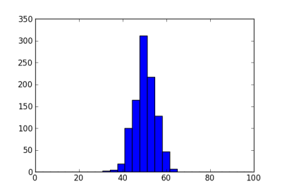
Suppose we have 100 patients to enroll in a clinical trial. If we assign each patient to a treatment arm with probability 1/2, there will be about 50 patients on each treatment. The following histogram shows the number of patients assigned to the first treatment arm in 1000 simulations. The standard deviation is about 5.

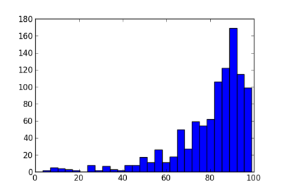
Next we let the randomization probability vary. Suppose the true probability of response is 50% on one arm and 70% on the other. We model the probability of response on each arm as a beta distribution, starting from a uniform prior. We randomize to an arm with probability equal to the posterior probability that that arm has higher response. The histogram below shows the number of patients assigned to the better treatment in 1000 simulations.

The standard deviation in the number of patients is now about 17. Note that while most trials assign 50 or more patients to the better treatment, some trials in this simulation put less than 20 patients on this treatment. Not only will these trials treat patients less effectively, they will also have low statistical power (as will the trials that put nearly all the patients on the better arm).

The reason for this volatility is that the method can easily be mislead by early outcomes. With one or two early failures on an arm, the method could assign more patients to the other arm and not give the first arm a chance to redeem itself.

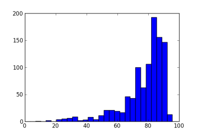
Because of this dynamic, various methods have been proposed to add “ballast” to adaptive randomization. See a comparison of three such methods here. These methods reduce the volatility in adaptive randomization, but do not eliminate it. For example, the following histogram shows the effect of adding a burn-in period to the example above, randomizing the first 20 patients equally.

The standard deviation is now 13.8, less than without the burn-in period, but still large compared to a standard deviation of 5 for equal randomization.

Another approach is to transform the randomization probability. If we use an exponential tuning parameter of 0.5, the sample standard deviation of the number of patients on the better arm is essentially the same, 13.4. If we combine a burn-in period of 20 and an exponential parameter of 0.5, the sample standard deviation is 11.7, still more than twice that of equal randomization.

Related