Mental math trick and deeper issues

I’d like to do two things in this post. I’ll present a fun bit of mental math, then use it to illustrate a few deeper points.

The story starts with a Twitter thread I wrote on @AlgebraFact.

The Fibonacci series begins

1, 1, 2, 3, 5, 8, 13, 21, ….

So this gives us a sequence of possible conversion factors:

1/1, 1/2, 2/3, 3/5, 5/8, 8/13, 13/21, ….

Which conversion factor is best?

“Best” depends on one’s optimization criteria. A lot of misunderstandings boil down to implicitly assuming everyone has the same optimization criteria in mind when they do not.

For the purposes of mentally approximating the width of the Strait of Gibraltar, 8/13 is ideal because the resulting arithmetic is trivial. Accuracy is not an issue here: surely the Strait is not exactly 13 kilometers wide. There’s probably more error in the 13 km statement than there is in the conversion to miles.

But what if accuracy were an issue?

The reason consecutive Fibonacci ratios make good conversion factors between miles and kilometers is that

Fn+1 / Fn → φ = 1.6180 …

as n grows, where φ is the golden ratio. We’re wanting to convert from kilometers to miles, so we actually want the conjugate golden ratio

1/φ = φ – 1 = 0.6180 …

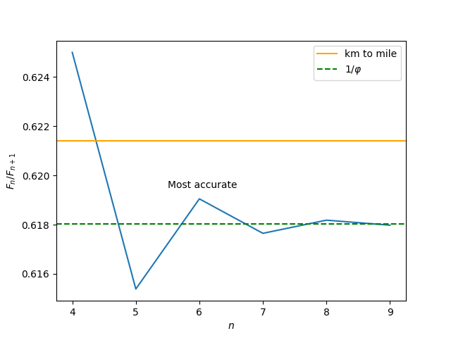
This is very close to the number of miles in a kilometer, which is 0.6214.

So back to our question: which conversion factor is best, if by best we mean most accurate?

The further out we go in the Fibonacci sequence, the closer the ratio of consecutive numbers is to the golden ratio, so we should go out as far as possible.

Except that’s wrong. We’ve committed a common error: optimizing a proxy. We don’t want to get as close as possible to the golden ratio; we want to get as close as possible to the conversion factor. The golden ratio was a proxy.

Initially, getting closer to our proxy got us closer to our actual goal. As we progress through the sequence

1/1, 1/2, 2/3, 3/5, 5/8, 8/13, 13/21

we get closer to 1/φ = 0.6180 and closer to our conversion factor 0.6214. But after 13/21 our goals diverge. Going further brings us closer to 1/φ but further from our conversion factor as the following plot illustrates.

Optimizing a proxy is not an error per se, but reification is. This is when you lose sight of your goal and forget that a proxy is a proxy. Optimizing a proxy is a practical expedient, and may be sufficient, but you have to remain aware that that’s what you’re doing.

For more along these lines, see the McNamara fallacy.

Physical versus medical modeling

Modeling is more fun when you have some confidence in your modeling assumptions. I’ve been working with models of physical systems lately and it’s been more enjoyable than the biostatistical modeling I’ve done over the last few years.

I have more confidence that my results might reflect reality. I also have more confidence that if my results don’t reflect reality, I’ll find out.

Related posts

Data calls the model’s bluff

I hear a lot of people saying that simple models work better than complex models when you have enough data. For example, here’s a tweet from Giuseppe Paleologo this morning:

Isn’t it ironic that almost all known results in asymptotic statistics don’t scale well with data?

There are several things people could mean when they say that complex models don’t scale well.

First, they may mean that the implementation of complex models doesn’t scale. The computational effort required to fit the model increases disproportionately with the amount of data.

Second, they could mean that complex models aren’t necessary. A complex model might do even better than a simple model, but simple models work well enough given lots of data.

A third possibility, less charitable than the first two, is that the complex models are a bad fit, and this becomes apparent given enough data. The data calls the model’s bluff. If a statistical model performs poorly with lots of data, it must have performed poorly with a small amount of data too, but you couldn’t tell. It’s simple over-fitting.

I believe that’s what Giuseppe had in mind in his remark above. When I replied that the problem is modeling error, he said “Yes, big time.” The results of asymptotic statistics scale beautifully when the model is correct. But giving a poorly fitting model more data isn’t going to make it perform better.

The wrong conclusion would be to say that complex models work well for small data. I think the conclusion is that you can’t tell that complex models are not working well with small data. It’s a researcher’s paradise. You can fit a sequence of ever more complex models, getting a publication out of each. Evaluate your model using simulations based on your assumptions and you can avoid the accountability of the real world.

If the robustness of simple models is important with huge data sets, it’s even more important with small data sets.

Model complexity should increase with data, not decrease. I don’t mean that it should necessarily increase, but that it could. With more data, you have the ability to test the fit of more complex models. When people say that simple models scale better, they may mean that they haven’t been able to do better, that the data has exposed the problems with other things they’ve tried.

Related posts

Floating point error is the least of my worries

“Nothing brings fear to my heart more than a floating point number.” — Gerald Jay Sussman

The context of the above quote was Sussman’s presentation We really don’t know how to compute. It was a great presentation and I’m very impressed by Sussman. But I take exception to his quote.

I believe what he meant by his quote was that he finds floating point arithmetic unsettling because it is not as easy to rigorously understand as integer arithmetic. Fair enough. Floating point arithmetic can be tricky. Things can go spectacularly bad for reasons that catch you off guard if you’re unprepared. But I’ve been doing numerical programming long enough that I believe I know where the landmines are and how to stay away from them. And even if I’m wrong, I have bigger worries.

Nothing brings fear to my heart more than modeling error.

The weakest link in applied math is often the step of turning a physical problem into a mathematical problem. We begin with a raft of assumptions that are educated guesses. We know these assumptions can’t be exactly correct, but we suspect (hope) that the deviations from reality are small enough that they won’t invalidate the conclusions. In any case, these assumptions are usually far more questionable than the assumption that floating point arithmetic is sufficiently accurate.

Modeling error is usually several orders of magnitude greater than floating point error. People who nonchalantly model the real world and then sneer at floating point as just an approximation strain at gnats and swallow camels.

In between modeling error and floating point error on my scale of worries is approximation error. As Nick Trefethen has said, if computers were suddenly able to do arithmetic with perfect accuracy, 90% of numerical analysis would remain important.

To illustrate the difference between modeling error, approximation error, and floating point error, suppose you decide that the probability of something can be represented by a normal distribution. This is actually two assumptions: that the process is random, and that as a random variable it has a normal distribution. Those assumptions won’t be exactly true, so this introduces some modeling error.

Next we have to compute something about a normal distribution, say the probability of a normal random variable being in some range. This probability is given by an integral, and some algorithm estimates this integral and introduces approximation error. The approximation error would exist even if the steps in the algorithm could be carried out in infinite precision. But the steps are not carried out with infinite precision, so there is some error introduced by implementing the algorithm with floating point numbers.

For a simple example like this, approximation error and floating point error will typically be about the same size, both extremely small. But in a more complex example, say something involving a high-dimensional integral, the approximation error could be much larger than floating point error, but still smaller than modeling error. I imagine approximation error is often roughly the geometric mean of modeling error and floating point error, i.e. somewhere around the middle of the two on a log scale.

In Sussman’s presentation he says that people worry too much about correctness. Often correctness is not that important. It’s often good enough to produce a correct answer with reasonably high probability, provided the consequences of an error are controlled. I agree, but in light of that it seems odd to be too worried about inaccuracy from floating point arithmetic. I suspect he’s not that worried about floating point and that the opening quote was just an entertaining way to say that floating point math can be tricky.

More on floating point computing