Lambert W strikes again

I was studying a statistics paper the other day in which the author said to solve

t log( 1 + n/t ) = k

for t as part of an algorithm. Assume 0 < k < n.

Is this well posed?

First of all, can this equation be solved for t? Second, if there is a solution, is it unique?

It’s not hard to show that as a function of t, the left side approaches 0 as t approaches 0, and it approaches n as t goes to infinity. So there is a solution for all k between 0 and n. The restriction on k is necessary since the left side cannot exceed n.

With a little more work one can show that the derivative is always positive, so the left side is a monotonically increasing function, and so the solution given each value of k is unique.

Analytic solution

Now if we fix n, we can think of the equation above as defining t as a function of k. Can we solve for t exactly? I suspected that there might be a solution in terms of the Lambert W function because if you divide by t and exponentiate, you get an equation that smells like the equation

z = w exp(w)

defining the function W(z). It turns out this is indeed the case.

If we ask Mathematica

    Solve[t Log[1 + n/t] ==  k, t]

we get

t\to -\frac{k}{ W\left(-\cfrac{k \exp(-k/n)}{n}\right)+\cfrac{k}{n}}

Great! There’s a closed-form solution, if you accept using the W function as being closed form.

Problems with the solution

I found the solution in Mathematica, but I tested it in Python to make sure both platforms define W the same way.

    from numpy import log, exp
    from scipy.special import lambertw

    def f(t, n):
        return t*log(1 + n/t)

    def g(k, n):
        r = k/n
        return -k/(lambertw(-r*exp(-r)) + r)

    n, k = 10, 8
    t = g(k, n)
    print(f(t, n))

This should print k, so it prints 8, right? No, it prints 10.

What’s up with that?

If we look back at the equation for t above, we see that the W function is being evaluated at x exp(x) where x = –k/n, so we should get –k/n back since W(x exp(x)) = x by definition. But that means our denominator is zero, and so the equation doesn’t make sense!

Things are getting worse. At first we had a wrong value, but at least it was finite!

The problem is not a difference between Mathematica and Python.

Resolution

The problem is we’ve glossed over a branch cut of the W function. To make a long story short, we were using the principal branch of the W function, but we should have used a different branch.

Let’s go back to where I asked Mathematica

    Solve[t Log[1 + n/t] == k, t]

I ran the solution through TeXForm to get the TeX code that produced the image for the solution equation. I made a few aesthetic changes to the TeX, but it was essentially Mathematica’s output.

Without the TeXForm, Mathematica’s solution was in terms of ProductLog, not in terms of W; the TeXForm function turned ProductLog into W. If you look up ProductLog, it will tell you

ProductLog[z] gives the principal solution for w in z = wew.

The principal solution. So we should be on the alert for difficulties with branches. There are two real solutions to z = wew for some values of z, and we have to choose the right one. For example, if z = -0.1, the w could be -0.1118 or -3.5772.

Mathematica gave me the wrong branch. But to be fair, it did try to warn me.

Solve::ifun: Inverse functions are being used by Solve, so some solutions may not be found; use Reduce for complete solution information.

The solution is to use the -1 branch. In Mathematica’s notation, the branch comes before the argument. In SciPy, the branch comes second. So to fix the code above, we need to change

    lambertw(-r*exp(-r))

to

   lambertw(-r*exp(-r), -1)

and then the code will be correct.

If x is negative, and we use the -1 branch of W, then

W-1(x exp(x)) ≠ x

and so we’re not dividing by zero in our solution.

More posts with Lambert W

Bessel determinants

The Bessel functions J and Y are analogous to sine and cosine. Bessel functions come up in polar coordinates the way sines and cosines come up in rectangular coordinates. There are J and Y functions of various orders, conventionally written with a subscript ν.

Plotting Bessel functions J_3 and Y_3

I recently ran across a curious set of relations between these functions and their derivatives. Let’s start with the following terms defined by 2 by 2 determinants.

\begin{align*} p_\nu &= \begin{vmatrix} J_\nu(a) & J_\nu(b) \\ Y_\nu(a) & Y_\nu(b) \\ \end{vmatrix} \\ q_\nu &= \begin{vmatrix} J_\nu(a) & J'_\nu(b) \\ Y_\nu(a) & Y'_\nu(b) \\ \end{vmatrix} \\ r_\nu &= \begin{vmatrix} J'_\nu(a) & J_\nu(b) \\ Y'_\nu(a) & Y_\nu(b) \\ \end{vmatrix} \\ s_\nu &= \begin{vmatrix} J'_\nu(a) & J'_\nu(b) \\ Y'_\nu(a) & Y'_\nu(b) \\ \end{vmatrix} \end{align*}

There are a lot of symmetries in the definitions above. First, every term has a subscript ν, so you can ignore those for now.

Second, every determinant has J‘s on the top row and Y‘s on the bottom.

 \begin{vmatrix} J & J \\ Y & Y \\ \end{vmatrix}

Third, every determinant has a‘s in the first column and b‘s in the second.

 \begin{vmatrix} a & b \\ a & b \\ \end{vmatrix}

And finally, the primes, indicating derivatives, have the following pattern.

 \begin{align*} p &= \begin{vmatrix} \phantom{\cdot} & \phantom{\cdot} \\ \phantom{\cdot} & \phantom{\cdot} \\ \end{vmatrix} \\ q &= \begin{vmatrix} \phantom{\cdot} & \phantom{\cdot}' \\ \phantom{\cdot} & \phantom{\cdot}' \\ \end{vmatrix} \\ r &= \begin{vmatrix} \phantom{\cdot}' & \phantom{\cdot} \\ \phantom{\cdot}' & \phantom{\cdot} \\ \end{vmatrix} \\ s &= \begin{vmatrix} \phantom{\cdot}' & \phantom{\cdot}' \\ \phantom{\cdot}' & \phantom{\cdot}' \\ \end{vmatrix} \end{align*}

Now that we have all these definitions in place, there are several identities that the p’s, q’s, r’s, and s‘s satisfy. Some of them depend on the orders, and that’s why we included the ν subscripts. You can find various relations in A&S equation 9.1.32, but I wanted to point out one that’s particularly elegant, A&S equation 9.1.34:

\begin{vmatrix} p_\nu & q_\nu \\ r_\nu & s_\nu \end{vmatrix} = \frac{4}{\pi^2ab}

This equation, a determinant of terms defined by determinants, reduces to a simple form that depends only on where the Bessel functions are evaluated, i.e. a and b, but not on their order ν.

Python example

The Python code below will show how to call Bessel functions and their derivatives and will illustrate the equations above.

    from math import pi
    from scipy.special import jv, yv, jvp, yvp
    
    def example(n, a, b):
    
        ja = jv(n, a)
        jb = jv(n, b)
        ya = yv(n, a)
        yb = yv(n, b)
        
        jap = jvp(n, a)
        jbp = jvp(n, b)
        yap = yvp(n, a)
        ybp = yvp(n, b)
        
        p = ja  * yb  - jb  * ya
        q = ja  * ybp - jbp * ya
        r = jap * yb  - jb  * yap
        s = jap * ybp - jbp * yap
        
        print(p*s - q*r)
        print(4/(pi*pi*a*b))
    
    example(3, 16, 21)

This prints

    0.0012062045671706876
    0.0012062045671706878

The two results differ slightly in the last decimal place due to rounding error.

The order of a Bessel function can be any real number [1], and the arguments can be any complex number. Here’s another example with more general arguments.

    example(3.14, 16-3j, 21+1.2j)    

This prints

    (0.0011738907214344785 + 0.00015140286689885318j)
    (0.0011738907214345800 + 0.00015140286689880630j)

with the real and imaginary parts agreeing to 15 decimal places.

Related posts

[1] You can define Bessel functions with complex order, but SciPy doesn’t support that.

Broadcasting and functors

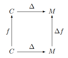
In my previous post, I looked at the map Δ that takes a column vector to a diagonal matrix. I even drew a commutative diagram, which foreshadows a little category theory.

Suppose you have a function f of a real or complex variable. To an R programmer, if x is a vector, it’s obvious that f(x) means to apply f to every component of a vector. Python (NumPy) works the same way, and calls this broadcasting. To a mathematician, this looks odd. What does the logarithm of a vector, for example, even mean?

As in the previous post, we can use Δ to formalize things. We said that Δ has some nice properties, and in fact we will show it is a functor.

To have a functor, we have to have categories. (Historically, functors came first; categories were defined in order to define functors.) We will define C to be the category of column vectors and M the category of square matrices as before. Or rather, we should say the objects of C are column vectors and the objects of M are square matrices.

Categories need morphisms, functions between objects [1]. We define the morphisms on C to be analytic functions applied componentwise. So, for example, if

z = [1, 2, -3],

then

tan(z) = [tan(1), tan(2), tan(-3)].

The morphisms on M will be analytic functions on square matrices, not applied componentwise but applied by power series. That is, given an analytic function f, we define f of a square matrix X as the result of sticking the matrix X into the power series for f. For an example, see What is the cosine of a matrix?

We said that Δ is a functor. It takes column vectors and turns them into square matrices by putting their contents along the diagonal of a matrix. We gave the example in the previous post that [4, i, π] would be mapped to the matrix with these elements on the diagonal, i.e.

\Delta: \begin{pmatrix} 4 \\ i \\ \pi \end{pmatrix} \mapsto \begin{pmatrix} 4 & 0 & 0\\ 0 & i & 0 \\ 0 & 0 & \pi \end{pmatrix}

That says what Δ does on objects, but what does it do on morphisms? It takes an analytic function that was applied componentwise to column vectors, and turns it into a function that is applied via its power series to square matrices. That is, starting with a function

f(z) = \sum_{n=0}^\infty a_nz^n

we define the morphism f on C by

f : \begin{pmatrix} z_1 \\ z_2 \\ \vdots \\ z_n \end{pmatrix} \mapsto \begin{pmatrix} f(z_1) \\ f(z_2) \\ \vdots \\ f(z_n) \end{pmatrix}

and the morphism Δ f on M by

\Delta f : Z \mapsto \sum_{n=0}^\infty a_n Z^n

where Z is a square matrix.

We can apply f to a column vector, and then apply Δ to turn the resulting vector into a diagonal matrix, or we could apply Δ to turn the vector into a diagonal matrix first, and then apply f (technically,  Δf). That is, the follow diagram commutes:

\begin{diagram}   C & \rTo^{\Delta} & M \\   \uTo^{f} & & \uTo_{\Delta f} \\   C & \rTo^{\Delta} & M  \end{diagram}

Python example

Applying an analytic function to a diagonal matrix gives the same result as simply applying the function to the elements of the diagonal. But for more general square matrices, this is not the case. We will illustrate this with some Python code.

    import numpy as np
    from scipy.linalg import funm

    d = np.array([1, 2])
    D = np.diag(d)
    M = np.array([[1, np.pi], [2, 0]])

Now let’s look at some output.

    >>> np.sin(d)                     
    array([0.84147098, 0.90929743])   

    >>> np.sin(D)                     
    array([[0.84147098, 0.        ],  
           [0.        , 0.90929743]]) 

    >>> funm(D, np.sin)               
    array([[0.84147098, 0.        ],  
           [0.        , 0.90929743]]) 

So if we take the sine of d and turn the result into a matrix, we get the same thing as if we turn d into a matrix D and then take the sine of D, either componentwise or as an analytic function (with funm, function of a matrix).

Now let’s look at a general, non-diagonal matrix.

    >>> np.sin(M)
    array([[0.84147099, 0],
       [0.90929743, 0]])

    >>> funm(D, np.sin)
    array([[0.84147098, 0.        ],
           [0.        , 0.90929743]])

Note that the elements in the bottom row are in opposite positions in the two examples.

[1] OK, morphisms are not necessarily functions, but in practice they usually are.

Python and the Tell-Tale Heart

I was browsing through SciPy documentation this evening and ran across a function in scipy.misc called electrocardiogram. What?!

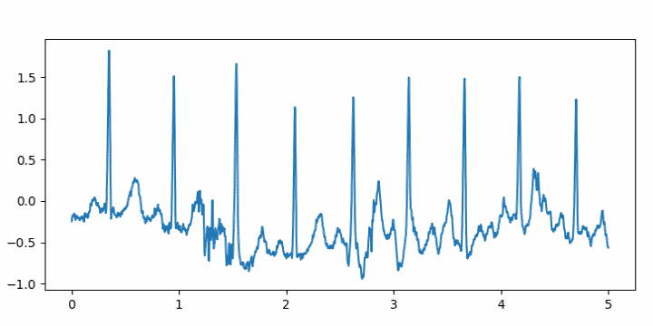
It’s an actual electrocardiogram, sampled at 360 Hz. Presumably it’s included as convenient example data. Here’s a plot of the first five seconds.

ECG plot

I wrote a little code using it to turn the ECG into an audio file.

from numpy import int16, iinfo
from scipy.io.wavfile import write
from scipy.misc import electrocardiogram

def to_integer(signal):
    # Take samples in [-1, 1] then scale to 16-bit integers
    m = iinfo(int16).max
    M = max(abs(signal))
    return int16(signal*m/M)

ecg = electrocardiogram()
write("heartbeat.wav", 360, to_integer(ecg))

I had to turn the volume way up to hear it, and that made me think of Edgar Allan Poe’s story The Tell-Tale Heart.

I may be doing something wrong. According to the documentation for the write function, I shouldn’t need to convert the signal to integers. I should just be able to leave the signal as floating point and normalize it to [-1, 1] by dividing by the largest absolute value in the signal. But when I do that, the output file will not play.

Related posts

Stable and unstable recurrence relations

Mother helping her toddler to walk

The previous post looked at computing recurrence relations. That post ends with a warning that recursive evaluations may nor may not be numerically stable. This post will give examples that illustrate stability and instability.

There are two kinds of Bessel functions, denoted J and Y. These are called Bessel functions of the first and second kinds respectively. These functions carry a subscript n denoting their order. Both kinds of Bessel functions satisfy the same recurrence relation:

fn+1 – (2n/x) fn + fn-1 = 0

where f is J or Y.

If you apply the recurrence relation in the increasing direction, it is unstable for J but stable for Y.

If you apply the recurrence relation in the opposite direction, it is stable for J and unstable for Y.

We will illustrate the above claims using the following Python code. Since both kinds of Bessel function satisfy the same recurrence, we pass the Bessel function in as a function argument. SciPy implements Bessel functions of the first kind as jv and Bessel functions of the second kind as yv. [1]

    from scipy import exp, pi, zeros
    from scipy.special import jv, yv

    def report(k, computed, exact):
        print(k, computed, exact, abs(computed - exact)/exact)

    def bessel_up(x, n, f):
        a, b = f(0, x), f(1, x)
        for k in range(2, n+1):
            a, b = b, 2*(k-1)*b/x - a
            report(k, b, f(k,x))     

    def bessel_down(x, n, f):
        a, b = f(n,x), f(n-1,x)
        for k in range(n-2, -1, -1):
            a, b = b, 2*(k+1)*b/x - a
            report(k, b, f(k,x))

We try this out as follows:

    bessel_up(1, 20, jv)
    bessel_down(1, 20, jv)
    bessel_up(1, 20, yv)
    bessel_down(1, 20, yv)

When we compute Jn(1) using bessel_up, the relative error starts out small and grows to about 1% when n = 9. The relative error increases rapidly from there. When n = 10, the relative error is 356%.

For n = 20, the recurrence gives a value of 316894.36 while the true value is 3.87e-25, i.e. the computed value is 30 orders of magnitude larger than the correct value!

When we use bessel_down, the results are correct to full precision.

Next we compute Yn(1) using bessel_up the results are correct to full precision.

When we compute Yn(1) using bessel_down, the results are about as bad as computing Jn(1) using bessel_up. We compute Y0(1) as 0 5.7e+27 while the correct value is roughly 0.088.

There are functions, such as Legendre polynomials, whose recurrence relations are stable in either direction, at least for some range of inputs. But it would be naive to assume that a recurrence is stable without some exploration.

Miller’s algorithm

There is a trick for using the downward recurrence for Bessel functions known as Miller’s algorithm. It sounds crazy at first: Assume JN(x) = 1 and JN+1(x) = 0 for some large N, and run the recurrence downward.

Since we don’t know JN(x) our results be off by some constant proportion. But there’s a way to find out what that proportionality constant is using the relation described here.

1 = J_0(x) + 2J_2(x) + 2J_4(x) + 2J_6(x) + \cdots

We add up out computed values for the terms on the right side, then divide by the sum to normalize our estimates. Miller’s recurrence algorithm applies more generally to other recurrences where the downward recurrence is stable and there exists a normalization identity analogous to the one for Bessel functions.

The following code lets us experiment with Miller’s algorithm.

    def miller(x, N):
        j = zeros(N) # array to store values
        
        a, b = 0, 1
        for k in range(N-1, -1, -1):
            a, b = b, 2*(k+1)*b/x - a
            j[k] = b
            
        norm = j[0] + sum(2*j[k] for k in range(2,N,2))
        j /= norm
        
        for k in range(N-1, -1, -1):
            expected, computed = j[k], jv(k,x)
            report(k, j[k], jv(k,x))

When we call miller(pi, 20) we see that Miller’s method computes Jn(π) accurately. The error starts out moderately small and decreases until the results are accurate to floating point precision.

    |----+------------|
    |  k | rel. error |
    |----+------------|
    | 19 |   3.91e-07 |
    | 17 |   2.35e-09 |
    | 16 |   2.17e-11 |
    | 15 |   2.23e-13 |
    | 14 |   3.51e-15 |
    |----+------------|

For smaller k the relative error is also around 10-15, i.e. essentially full precision.

[1] Why do the SciPy names end in “v”? The order of a Bessel function does not have to be an integer. It could be any real number, and the customary mathematical notation is to use a Greek letter ν (nu) as a subscript rather than n as a reminder that the subscript might not represent an integer. Since a Greek ν looks similar to an English v, SciPy uses v as a sort of approximation of ν.

Area of sinc and jinc function lobes

Someone left a comment this morning on my blog post on sinc and jinc integrals regarding the area of the lobes.

It would be nice to have the values of integrals of each lobe, i.e. integrals between 0 and multiples of pi. Anyone knows of such a table?

This post will include Python code to address that question. (Update: added asymptotic approximation. See below.)

First, let me back up and explain the context. The sinc function is defined as [1]

sinc(x) = sin(x) / x

and the jinc function is defined analogously as

jinc(x) = J1(x) / x,

substituting the Bessel function J1 for the sine function. You could think of Bessel functions as analogs of sines and cosines. Bessel functions often come up when vibrations are described in polar coordinates, just as sines and cosines come up when using rectangular coordinates.

Here’s a plot of the sinc and jinc functions:

The lobes are the regions between crossings of the x-axis. For the sinc function, the lobe in the middle runs from -π to π, and for n > 0 the nth lobe runs from nπ to (n+1)π. The zeros of Bessel functions are not uniformly spaced like the zeros of the sine function, but they come up in application frequently and so it’s easy to find software to compute their locations.

First of all we’ll need some imports.

    from scipy import sin, pi
    from scipy.special import jn, jn_zeros
    from scipy.integrate import quad

The sinc and jinc functions are continuous at zero, but the computer doesn’t know that [2]. To prevent division by zero, we return the limiting value of each function for very small arguments.

    def sinc(x):
        return 1 if abs(x) < 1e-8 else sin(x)/x

    def jinc(x):
        return 0.5 if abs(x) < 1e-8 else jn(1,x)/x

You can show via Taylor series that these functions are exact to the limits of floating point precision for |x| < 10-8.

Here’s code to compute the area of the sinc lobes.

    def sinc_lobe_area(n):
        n = abs(n)
        integral, info = quad(sinc, n*pi, (n+1)*pi)
        return 2*integral if n == 0 else integral

The corresponding code for the jinc function is a little more complicated because we need to compute the zeros for the Bessel function J1. Our solution is a little clunky because we have an upper bound N on the lobe number. Ideally we’d work out an asymptotic value for the lobe area and compute zeros up to the point where the asymptotic approximation became sufficiently accurate, and switch over to the asymptotic formula for sufficiently large n.

    def jinc_lobe_area(n):
        n = abs(n)
        assert(n < N)
        integral, info = quad(jinc, jzeros[n-1], jzeros[n])
        return 2*integral if n == 0 else integral

Note that the 0th element of the array returned by jn_zeros is the first positive zero of J1; it doesn’t include the zero at the origin.

For both sinc and jinc, the even numbered lobes have positive area and the odd numbered lobes have negative area. Here’s a plot of the absolute values of the lobe areas.

Asymptotic results

We can approximate the area of the nth lobe of the sinc function by using a midpoint approximation for 1/x. It works out that the area is asymptotically equal to

 (-1)^n \frac{4}{(2n+1)\pi}

We can do a similar calculation for the area of the nth jinc lobe, starting with the asymptotic approximation for jinc given here. We find that the area of the nth lobe of the jinc function is asymptotically equal to

\frac{(-1)^n}{\pi^2} \left( \frac{8}{4n+3} \right )^{3/2}

To get an idea of the accuracy of the asymptotic approximations, here are the results for n=100.

    sinc area:      0.00633455
    asymptotic:     0.00633452
    absolute error: 2.97e-8
    relative error: 4.69e-6

    jinc area:      0.000283391
    asymptotic:     0.000283385
    absolute error: 5.66e-9
    relative error: 2.00e-5

More signal processing posts

[1] Some authors define sinc(x) as sin(πx)/πx. Both definitions are common.

[2] Scipy has a sinc function in scipy.special, defined as sin(πx)/πx, but it doesn’t have a jinc function.

Calculating the period of Van der Pol oscillators

A few days ago I wrote about how to solve differential equations with SciPy’s ivp_solve function using Van der Pol’s equation as the example. Van der Pol’s equation is

{d^2x \over dt^2}-\mu(1-x^2){dx \over dt}+x= 0

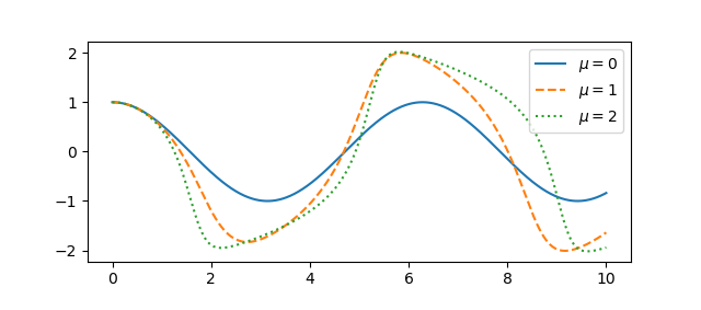
The parameter μ controls the amount of nonlinear damping. For any initial condition, the solution approach a periodic solution. The limiting periodic function does not depend on the initial condition [1] but does depend on μ. Here are the plots for μ  = 0, 1, and 2 from the previous post.

Van der Pol oscillator solutions as a function of time

A couple questions come to mind. First, how quickly do the solutions become periodic? Second, how does the period depend on μ? To address these questions, we’ll use an optional argument to ivp_solve we didn’t need in the earlier post.

Using events in ivp_solve

For ivp_solve an event is a function of the time t and the solution y whose roots the solver will report. To determine the period, we’ll look at where the solution is zero; our event function is trivial since we want to find the roots of the solution itself.

Recall from the earlier post that we cast our second order ODE as a pair of first order ODEs, and so our solution is a vector, the function x and its derivative. So to find roots of the solution, we look at what the solver sees as the first component of the solver. So here’s our event function:

    def root(t, y): return y[0]

Let’s set μ = 2 and find the zeros of the solution over the interval [0, 40], starting from the initial condition x(0) = 1, x‘(0) = 0.

    mu = 2
    sol = solve_ivp(vdp, [0, 40], [1, 0], events=root)
    zeros = sol.t_events[0]

Here we reuse the vdp function from the previous post about the Van der Pol oscillator.

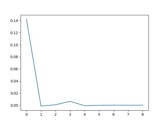
To estimate the period of the limit cycle we look at the spacing between zeros, and how that spacing is changing.

    spacing = zeros[1:] - zeros[:-1]
    deltas = spacing[1:] - spacing[:-1]

If we plot the deltas we see that the zero spacings quickly approach a constant value. Zero crossings are half periods, so the period of the limit cycle is twice the limiting spacing between zeros.

Van der pol period deltas

Theoretical results

If μ = 0 the Van der Pol oscillator reduces to a simple harmonic oscillator and the period is 2π. As μ increases, the period increases.

For relatively small μ we can calculate the period as above, but as μ increases this becomes more difficult numerically [2]. But one can easily show that the period is asymptotically

T ~ (3 – 2 log 2) μ

as μ goes to infinity. A more refined estimate due to Mary Cartwright is

T ~ (3 – 2 log 2) μ + 2π/μ1/3

for large μ.

More VdP posts

[1] There is a trivial solution, x = 0, corresponding to the initial conditions x(0) = x‘(0) = 0. Otherwise, every set of initial conditions leads to a solution that converges to the periodic attractor.

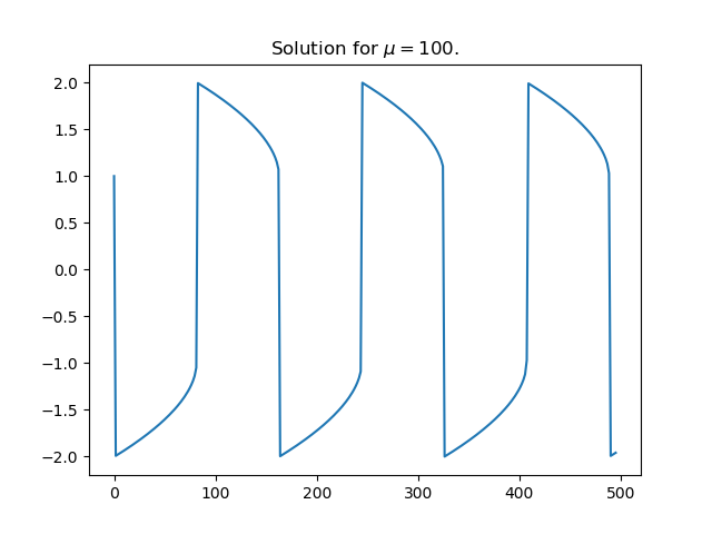
[2] To see why large values of μ are a problem numerically, here’s a plot of a solution for μ = 100.

Solution to Van der Pol for large damping parameter mu

The solution is differentiable everywhere, but the derivative changes so abruptly at the maxima and minima that it is discontinuous for practical purposes.

Solving Van der Pol equation with ivp_solve

Van der Pol’s differential equation is

{d^2x \over dt^2}-\mu(1-x^2){dx \over dt}+x= 0

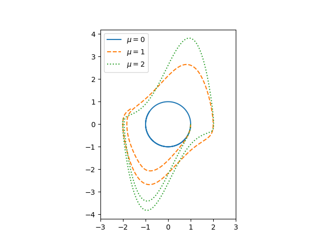
The equation describes a system with nonlinear damping, the degree of nonlinearity given by μ. If μ = 0 the system is linear and undamped, but as μ increases the strength of the nonlinearity increases. We will plot the phase portrait for the solution to Van der Pol’s equation in Python using SciPy’s new ODE solver ivp_solve.

The function ivp_solve does not solve second-order systems of equations directly. It solves systems of first-order equations, but a second-order differential equation can be recast as a pair of first-order equations by introducing the first derivative as a new variable.

\begin{align*} {dx \over dt} &= y \\ {dy \over dt}&= \mu(1-x^2)y -x \\ \end{align*}

Since y is the derivative of x, the phase portrait is just the plot of (x, y).

Phase portait of Van der Pol oscillator

If μ = 0, we have a simple harmonic oscillator and the phase portrait is simply a circle. For larger values of μ the solutions enter limiting cycles, but the cycles are more complicated than just circles. These limiting cycles are periodic attractors: every non-trivial solution converges to the limit cycle.

Here’s the Python code that made the plot.

from scipy import linspace
from scipy.integrate import solve_ivp
import matplotlib.pyplot as plt

def vdp(t, z):
    x, y = z
    return [y, mu*(1 - x**2)*y - x]

a, b = 0, 10

mus = [0, 1, 2]
styles = ["-", "--", ":"]
t = linspace(a, b, 500)

for mu, style in zip(mus, styles):
    sol = solve_ivp(vdp, [a, b], [1, 0], t_eval=t)
    plt.plot(sol.y[0], sol.y[1], style)
  
# make a little extra horizontal room for legend
plt.xlim([-3,3])    
plt.legend([f"$\mu={m}$" for m in mus])
plt.axes().set_aspect(1)

To plot the solutions as a function of time, rather than plotting phase portraits, change the line

    plt.plot(sol.y[0], sol.y[1], style)

to

    plt.plot(sol.t, sol.y[0], style)

and comment out the line setting xlim This gives the following plot.

Van der Pol oscillator solutions as a function of time

More dynamical system posts

Illustrating Cayley-Hamilton with Python

If you take a square matrix M, subtract x from the elements on the diagonal, and take the determinant, you get a polynomial in x called the characteristic polynomial of M. For example, let

M = \left[ \begin{matrix} 5 & -2 \\ 1 & \phantom{-}2 \end{matrix} \right]

Then

\left| \begin{matrix} 5-x & -2 \\ 1 & 2-x \end{matrix} \right| = x^2 - 7x + 12

The characteristic equation is the equation that sets the characteristic polynomial to zero. The roots of this polynomial are eigenvalues of the matrix.

The Cayley-Hamilton theorem says that if you take the original matrix and stick it into the polynomial, you’ll get the zero matrix.

\left[ \begin{matrix} 5 & -2 \\ 1 & \phantom{-}2 \end{matrix} \right]^2 - 7\left[ \begin{matrix} 5 & -2 \\ 1 & \phantom{-}2 \end{matrix} \right] + 12\left[ \begin{matrix} 1 & 0 \\ 0 & 1\end{matrix} \right] = \left[ \begin{matrix} 0 & 0 \\ 0 & 0\end{matrix} \right]

In brief, a matrix satisfies its own characteristic equation. Note that for this to hold we interpret constants, like 12 and 0, as corresponding multiples of the identity matrix.

You could verify the Cayley-Hamilton theorem in Python using scipy.linalg.funm to compute a polynomial function of a matrix.

>>> from scipy import array
>>> from scipy.linalg import funm
>>> m = array([[5, -2], [1, 2]])
>>> funm(m, lambda x: x**2 - 7*x + 12)

This returns a zero matrix.

I imagine funm is factoring M into something like PDP-1 where D is a diagonal matrix. Then

f(M) = P f(D) P-1.

This is because f can be applied to a diagonal matrix by simply applying f to each diagonal entry independently. You could use this to prove the Cayley-Hamilton theorem for diagonalizable matrices.

Related posts

Data Science and Star Science

I recently got a review copy of Statistics, Data Mining, and Machine Learning in Astronomy. I’m sure the book is especially useful to astronomers, but those of us who are not astronomers could use it as a survey of data analysis techniques, especially using Python tools, where all the examples happen to come from astronomy. It covers a lot of ground and is pleasant to read.