Maxwell-Boltzmann and Gamma

Posted on 7 January 2023 by John

When I shared an image from the previous post on Twitter, someone who goes by the handle Nonetheless made the astute observation that image looked like the Maxwell-Boltzmann distribution. That made me wonder what 1/Γ(x) would be like turned into a probability distribution, and whether it would be approximately like the Maxwell-Boltzmann distribution.

(Here I’m looking at something related to what Nonetheless said, but different. He was looking at my plot of the error in approximating 1/Γ(x) by partial products, but I’m looking at 1/Γ(x) itself.)

Making probability distributions

You can make any non-negative function with a finite integral into a probability density function by dividing it by its integral. So we can define a probability density function

$f(x) = \frac{c}{\Gamma(x)}$

where

$1/c = \int_0^\infty \frac{dx}{\Gamma(x)}$

and so c = 0.356154. (The integral cannot be computed in closed form and so has to be evaluated numerically.)

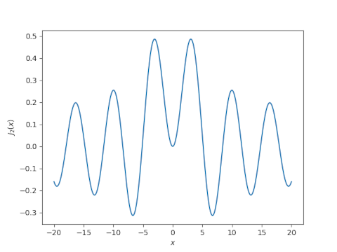
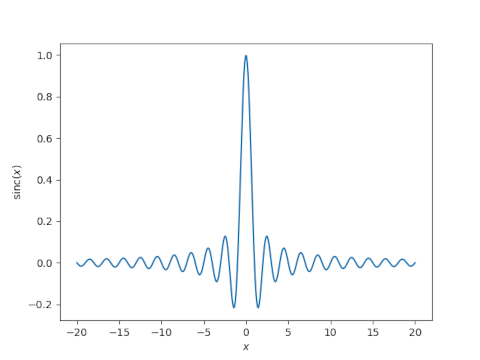
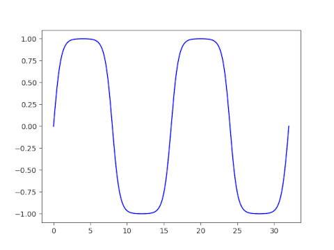
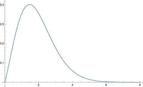
Here’s a plot of f(x).

Note that we’re doing something kind of odd here. It’s common to see the gamma function in the definition of probability distributions, but the function is always evaluated at distribution parameters, not at the free variable x. We’ll give an example of this shortly.

Maxwell-Boltzmann distribution

The Maxwell-Boltzmann distribution, sometimes called just the Maxwell distribution, is used in statistical mechanics to give a density function for particle velocities. In statistical terminology, the Maxwell-Boltzmann distribution is a chi distribution [1] with three degrees of freedom and a scale parameter σ that depends on physical parameters.

The density function for a Maxwell-Boltzmann distribution with k degrees of freedom and scale parameter σ has the following equation.

$\chi(x; k, \sigma) = \frac{1}{2^{(k/2) -1}\sigma \Gamma(k/2)} \left(\frac{x}{\sigma}\right)^{k-1} \exp(-x^2/2\sigma^2)$

Think of this as x^k-1 exp(-x² / 2σ²) multiplied by whatever you have to multiply it by to make it integrate to 1; most of the complexity in the definition is in the proportionality constant. And as mentioned above, the gamma function appears in the proportionality constant.

For the Maxwell-Boltzmann distribution, k = 3.

Lining up distributions

Now suppose we want to compare the distribution we’ve created out of 1/Γ(x) with the Maxwell-Boltzman distribution. One way of to do this would be to align the two distributions to have their peaks at the same place. The mode of a chi random variable with k degrees of freedom and scale σ is

$x = \sqrt{k-1} \, \sigma$

and so for a given k we can solve for σ to put the mode where we’d like.

For positive values, the minimum of the gamma function, and hence the maximum of its reciprocal, occurs at 1.46163. As with the integral above, this has to be computed numerically.

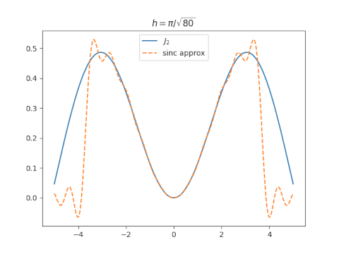
For the Maxwell-Boltzmann distribution, i.e. when k = 3, we don’t get a very good fit.

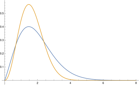
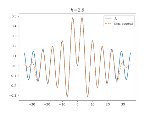
The tails on the chi distribution are too thin. If we try again with k = 2 we get a much better fit.

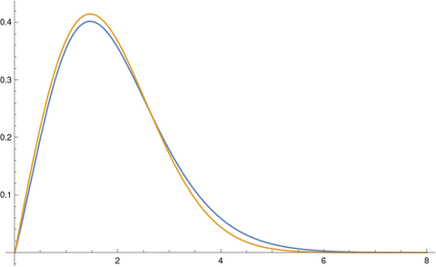
You get an even better fit with k = 1.86. The optimal value of k would depend on your criteria for optimality, but k = 1.86 looks like a good value just eyeballing it.

[1] This is a chi distribution, not the far more common chi-square distribution. The first time you see this is looks like a typo. If X is a random variable with a chi random variable with k degrees of freedom then X² has a chi-square distribution with k degrees of freedom.

Visualizing convergence of an infinite product

Posted on 7 January 2023 by John

A little while ago I wrote a post looking at how the infinite product for sine converges. The plot of the error terms is both mathematically and aesthetically interesting.

This post will look at similar plots for the reciprocal of the gamma function.

The reciprocal of the gamma function is an entire function, i.e. is analytic everywhere in the complex plane, and so it has an infinite product representation.

$\frac{1}{\Gamma (z)} = z\exp(\gamma z)\prod_{n=1}^{\infty }\left ( 1+\frac{z}{n} \right )\exp(-z/n)$

To visualize the convergence, we’ll take the product of the first N terms in the infinite product and subtract 1/Γ(z). We’ll plot these differences letting N range from 5 to 25.

Here’s the plot for -2 ≤ z ≤ 0.

And here’s the plot for 0 ≤ z ≤ 10.

Sinc approximation to Bessel function

Posted on 29 December 2022 by John

The Bessel functions J_n for even n look something like the sinc function. How well can you approximate the former by sums of the latter? To make things concrete, we’ll approximate J₂. Here’s a plot of J₂.

J_2

And here’s a plot of sinc(x) = sin(πx)/πx.

sinc(x)

The sinc approximation for a function f(x) is given by

$f(x) \approx \sum_{j=-n}^n f(jh) \, \text{sinc}\left(\frac{x - jh}{h}\right)$

Sinc approximation can be remarkably accurate, nearly optimal in some sense.

The accuracy of the approximation increases as n gets larger and h gets smaller. We will fix n = 10. How should we pick h? The paper cited in this post suggests using

$h = \frac{\pi}{2} \sqrt{\frac{1}{2n}} = 0.35124$

Let’s try that and see what happens.

The approximation isn’t very good overall, though it’s excellent near 0.

Before making plots, I had a plausible argument for why the value of h suggested above might be optimal. I also had an argument for why a much larger value of h, something on the order of 8 might be optimal. Turns out both are wrong. You can get a good approximation over a larger range by choosing h around 2.6.

Chebyshev series for sine

Posted on 26 December 2022 by John

In last week’s post on polynomial approximations for sine, I showed that the polynomial based on Chebyshev series was much better than a couple alternatives. I calculated a few terms of the Chebyshev series for sin(πx) but didn’t include the calculations in that blog post. I calculated the series coefficients numerically, but this post will show how to calculate the coefficients analytically.

Generalities

The Chebyshev series for a function f(x) on [-1, 1] is given by

$f(x) = \frac{a_0}{2} + \sum_{n=1}^\infty a_n T_n(x)$

where T_n(x) is the nth Chebyshev polynomial of the first kind. The coefficients are given by

$a_n = \frac{2}{\pi} \int_{-1}^1 \frac{f(x) \,T_n(x)}{\sqrt{1-x^2}} \, dx$

One way of defining the polynomials T_n(x) is

$T_n(\cos\theta) = \cos(n \theta)$

and so the change of variables x = cos θ lets us conclude

$a_n = \frac{2}{\pi} \int_0^\pi f(\cos \theta) \cos n\theta \, d\theta$

Series for sin(πx)

Now for our particular function, f(x) = sin(πx), we know by symmetry that the coefficients with even subscripts will be zero. This is because sine is an odd function, and T_n is an even function when n is even,

Using equation 10.9.2 here we can prove that if n = 2k+1 then

$a_n = (-1)^k 2 J_n(\pi)$

where J_n is the nth Bessel function of the first kind.

(The preceding sentence was the conclusion to a fair amount of fumbling around on my part. As is often the case in mathematics, the length of the write-up is unrelated to the length of the discovery process.)

Conformal map from rectangles to half plane

Posted on 12 December 2022 by John

As discussed in the previous post, the Jacobi elliptic function sn(z, m) is doubly periodic in the complex plane, with period 4K(m) in the horizontal direction and period 2K(1-m) in the vertical direction. Here K is the complete elliptic integral of the first kind.

The function sn(z, m) maps the rectangle

(-K(m), K(m)) × (0, K(1-m))

conformally onto to the upper half plane, i.e. points in the complex plane with non-negative imaginary part.

For example, sn(z, 0.5) takes the rectangle

The function sn has a singularity at the top middle of the rectangle, and so as horizontal lines approach the top of the rectangle, their image turns into bigger and bigger circles. filling the half plane.

The plot above was created with the following Mathematica code:

    K = EllipticK[1/2]
    Show[
        ParametricPlot[
            Table[{Re[JacobiSN[x + I y, 0.5]], Im[JacobiSN[x + I y, 0.5]]}, 
            {x, -K, K, K/10}], {y, 0, K}], 
        ParametricPlot[
             Table[{Re[JacobiSN[x + I y, 0.5]], Im[JacobiSN[x + I y, 0.5]]}, 
             {y, 0, K, K/10}], {x, -K, K}], 
        PlotRange -> {{-8, 8}, {0, 8}}]

You can vary the parameter m to match the shape of the rectangle you want to map to the half plane. You cannot choose both the length and width of your rectangle with only one parameter, but you can choose the aspect ratio. By choosing m = 1/2 we got a rectangle twice as wide as it is tall.

In our example we have a rectangle 3.70815 wide and 1.85407 tall. If we wanted a different size but the same aspect ratio, we could scale the argument to sn. For example,

sn(Kz, 0.5)

would map the rectangle (-1, 1) × (0, 1) onto the open half plane where K is given in the Mathematica code above.

In general we can solve for the parameter m that gives us the desired aspect ratio, as explained in the previous post, then find k such that sn(kz, m) maps the rectangle of the size we want into the half plane.

The inverse function, mapping the half plane to the rectangle, can be found in terms of elliptic integrals. Mathematica provides a convenient function InverseJacobiSN for this.

We could map any rectangle conformally to any other rectangle by mapping the first rectangle to the upper half plane, then mapping the upper half plane to the second rectangle. (We can’t simply scale the rectangle directly because such a map will not be conformal, will not preserve angles, unless we scale horizontally and vertically by the same amount. We can find a conformal map that will change the aspect ratio of a rectangle, but it will not simply scale the rectangle linearly.)

Although we can conformally map between any two rectangles using the process described above, we may not want to do things this way; the result may not be what we expect. Conformal maps between regions are not quite unique. They are unique if you specify where one point in the domain goes and specify the argument of its derivative. You may need to play with those extra degrees of freedom to get a conformal map that behaves as you expect.

Solve for Jacobi sn parameter to have given period(s)

Posted on 12 December 2022 by John

Here’s a calculation that I’ve had to do a few times. I’m writing it up here for my future reference and for the benefit of anybody else who needs to do the same calculation.

The Jacobi sn function is doubly periodic: it has one period as you move along the real axis and another period as you move along the imaginary axis. Its values are determined by a fundamental rectangle, and here we solve for a parameter 0 ≤ m < 1 that yields a desired length, or width, or aspect ratio for this rectangle.

You cannot specify both the length and width of the fundamental rectangle independently: you only have one degree of freedom. You can specify its length, or width, or aspect ratio.

This post focuses on sn, then explains how to modify the results for the other Jacobi elliptic functions—cn, dn, sc, etc.—at the end.

Given period

A parameter value m corresponds to a horizontal period of 4K(m) and a vertical period of 2K(1-m) where K is the complete elliptic integral of the first kind.

K(m) is an increasing function from [0, 1) to [π/2, ∞). So the minimum horizontal period is 2π and the minimum vertical period is π.

Given aspect ratio

The ratio of the horizontal period to the vertical period is given by

r(m) = 4K(m) / 2K(1-m) = 2K(m)/K(1-m).

The function r is an increasing function from [0, 1) to [0, ∞), so any aspect ratio is possible. This is important, for example, in conformal mapping. You cannot specify the length and width of the fundamental period independently, but you can solve for the parameter m that gives the aspect ratio you want, then follow it by a dilation to then get the length and width you want.

Numerical computation

If you need to find m efficiently or to high precision, see [1]. The code here simple and good enough for my purposes, and hopefully good enough for yours.

We need to either invert K or r, both of which are monotone functions, and so we can use the bisection method to find the value of m we’re after. The bisection method is not the most efficient, but it’s simple and very robust.

Python code

    from numpy import pi, linspace
    from scipy.special import ellipk, ellipj
    from scipy.optimize import bisect
    
    def invert_ellipk(K):
        "Given K, find m such that K(m) = K."
        assert(K >= pi/2)
        if K == pi/2:
            return 0
    
        # Find a bracket [a, b] for m
        a = 0
        b = 0.5
        y = ellipk(b)
        while y < K:
            b = 0.5*(b + 1)
            y = ellipk(b)
        return bisect(lambda m: ellipk(m)-K, a, b)
    
    def invert_horizontal_period(T):
        "Find parameter m such that sn(z, m) has real period T."
        return invert_ellipk(T/4)
    
    def invert_vertical_period(T):
        "Find parameter m such that sn(z, m) has imaginary period T."    
        return invert_ellipk(T/2)
    
    def invert_r(r):
        "Find parameter m such that the fundamental rectangle of sn(z, m) has aspect ratio r."
    
        ratio = lambda m: 2*ellipk(m)/ellipk(1-m)
        
        if r == 2:
            return 1/2
    
        a, b = 0.5, 0.5
        while ratio(b) < r: b = 0.5*(1 + b) while ratio(a) > r:
            a /= 2
        return bisect(lambda m: r - ratio(m), a, b)

To test the code, let’s find m such that sn(z, m) has period 5 along the real axis.

    import matplotlib.pyplot as plt

    T = 16
    m = invert_horizontal_period(T)
    print(4*ellipk(m))
    assert(abs(4*ellipk(m) - T) < 1e-8)
    x = linspace(0, 2*T, 200)
    plt.plot(x, sn(x, m))

This produces a plot that does have period 16.

Other Jacobi elliptic functions

There are 12 Jacobi elliptic functions, denoted with all pairs of {s, c, d, n} such that the two letters are different. The periods of the functions fall into three groups.

The functions sn, ns, cd, and dc all have real period 4K(m) and imaginary period 2K(1-m).

The functions cn, nc, ds, and sd all have real period 4K(m) and imaginary period 4K(1-m).

The functions cs, sc, dn, and nd all have real period 2K(m) and imaginary period 4K(1-m).

You can find plots of fundamental rectangles of these 12 functions here.

[1] Toshio Fukushima. Numerical computation of inverse complete elliptic integrals of the first and second kinds. Journal of Computational and Applied Mathematics. 249 (2013) 37–50.

Conformal map of ellipse interior to a disk

Posted on 27 November 2022 by John

This post will present the conformal map between the interior of an ellipse and the unit disk.

Given an ellipse centered at the origin with semi-major axis a and semi-minor axis b. Will will assume without loss of generality that a² – b² = 1 and so the foci are at ±1.

Hermann Schwarz published the conformal map from the ellipse to the unit disk in 1869 [1, 2].

The map is given by

$f(z) = \sqrt{k}\,\, \text{sn} \left( \frac{2K}{\pi} \sin^{-1}(z) \right)$

where sn is the Jacobi elliptic function with parameter k². The constants k and K are given by

$\begin{align*} q &= (a + b)^{-4} \\ k &= \left(\frac{\theta_2(q)}{\theta_3(q)}\right)^2 \\ K &= \frac{\pi}{2} \theta_3(q)^2 \end{align*}$

where θ₂ and θ₃ are theta constants, the value so the theta functions θ₂(z, q) and θ₃(z, q) at z = 1.

Conformal maps to the unit disk are unique up to rotation. The map above is the unique conformal map preserving orientation:

$\begin{align*} f(0) &= 0 \\ f(\pm a) &= \pm 1 \\ f(\pm bi) &= \pm i \\ \end{align*}$

Inverse map

The inverse of this map is given by

$g(w) = \sin\left(\frac{\pi}{2K} \,\, \text{sn}^{-1} \left(\frac{w}{\sqrt{k}}\right) \right)$

The inverse of the sn function with parameter m can be written in terms of elliptic integrals.

$\text{sn}^{-1}(z; m) = F\left(\sin^{-1}(u; m)\right)$

where F is the incomplete elliptic integral of the first kind and m is the parameter of sn and the parameter of F.

Plot

I wanted to illustrate the conformal map using an ellipse with aspect ratio 1/2. To satisfy a² – b² = 1, I set a = 2/√3 and b = 1/√3. The plot at the top of the post was made using Mathematica.

[1] H. A. Schwarz, Über eigige Abbildungsaufgaben, Journal für di reine und angew. Matheamatik, vol 70 (1869), pp 105–120

[2] Gabor Szegö. Conformal Mapping of the Interior of an Ellipse onto a Circle. The American Mathematical Monthly, 1950, Vol. 57, No. 7, pp. 474–478

Posts on ellipses and elliptic integrals

Posted on 21 November 2022 by John

I wrote a lot of posts on ellipses and related topics over the last couple months. Here’s a recap of the posts, organized into categories.

Basic geometry

More advanced geometry

Analysis

Calculating sine to an absurd number of digits

Posted on 18 November 2022 by John

Suppose you wanted to calculate sin(x) to a million decimal places using a Taylor series. How many terms of the series would you need?

You can use trig identities to reduce the problem to finding sin(x) for |x| ≤ 1. Let’s take the worst case and assume we want to calculate sin(1).

The series for sine alternates, and so by the alternating series theorem we need the first term left out of our Taylor approximation to be less than our error tolerate ε. If we keep the terms of the Taylor series up to x^{2m – 1} then we need

x^{2m + 1} / (2m + 1)! < ε.

Since we’re interested in x = 1 and Γ(n + 1) = n!, we need

1/ε < Γ(2m + 2).

That means we need

2m + 2 > Γ^-1(1/ε).

But how do you compute the inverse of the gamma function? This is something I wrote about a few years ago.

Here is a function for approximately computing the inverse of the gamma function. See the earlier post for details.

    from numpy import pi, e, sqrt, log
    from scipy.special import lambertw

    def inverse_gamma(x):
        c = 0.03653381448490056
        L = log((x+c)/sqrt(2*pi))
        return L / (lambertw(L/e)) + 0.5

Suppose we want to compute sin(1) to 100 decimal places. We need 2m + 2 to be larger than Γ^-1(10¹⁰⁰), and the code above tells us that Γ^-1(10¹⁰⁰) is something like 70.9. This tells us we can choose m = 35.

If we want to compute sin(1) to thousands of digits, the code above will fail because we cannot represent 10¹⁰⁰⁰ as a floating point number. I will assume for this post that we will use an extended precision library for summing the series for sin(1), but we’re going to use ordinary precision to plan this calculation, i.e. to decide how many terms to sum.

If we look closely at the function inverse_gamma above we see that it only depends on x via log(x + c). Since we’re interested in large x, we can ignore the difference between log(x + c) and log(x). This lets us write a new version of inverse_gamma that takes the log of x rather than x as an argument.

    def inverse_gamma2(logx):
        L = logx - log(sqrt(2*pi))
        return L/lambertw(L/e) + 0.5

Calling inverse_gamma with x = 10¹⁰⁰ gives the same result, down to the last decimal place, as calling inverse_gamma2 with 100 log(10).

We asked at the top of the post about computing sine to a million decimal places. If we call inverse_gamma2(1e6*log(10)) we get 205023.17… and so m = 102,511 would be large enough.

***

If you enjoyed reading this post, you may like reading this post on planning a world record calculation for computing ζ(3).

Entropy of a Student t distribution

Posted on 15 November 2022 by John

I was looking up the entropy of a Student t distribution and something didn’t seem right, so I wanted to look at familiar special cases.

The Student t distribution with ν degrees of freedom has two important special cases: ν = 1 and ν = ∞. When ν = 1 we get the Cauchy distribution, and in the limit as ν → ∞ we get the normal distribution. The expression for entropy is simple in these two special cases, but it’s not at all obvious that the general expression at ν = 1 and ν = ∞ gives the entropy for the Cauchy and normal distributions.

The entropy of a Cauchy random variable (with scale 1) is

$\log(4 \pi)$

and the entropy of a normal random variable (with scale 1) is

$(\log(2\pi) + 1)/2$

The entropy of a Student t random variable with ν degrees of freedom is

$\frac{\nu+1}{2} \left( \psi\left(\frac{\nu + 1}{2}\right) - \psi\left(\frac{\nu}{2}\right) \right) + \log\left( \sqrt{\nu} B\left(\frac{\nu}{2}, \frac{1}{2} \right) \right)$

Here ψ is the digamma function, the derivative of the log of the gamma function, and B is the beta function. These two functions are implemented as psi and beta in Python, and PolyGamma and Beta in Mathematica. Equation for entropy found on Wikipedia.

This post will show numerically and analytically that the general expression does have the right special cases. As a bonus, we’ll prove an asymptotic formula for the entropy along the way.

Numerical evaluation

Numerical evaluation shows that the entropy expression with ν = 1 does give the entropy for a Cauchy random variable.

    from numpy import pi, log, sqrt
    from scipy.special import psi, beta

    def t_entropy(nu):
        S = 0.5*(nu + 1)*(psi(0.5*(nu+1)) - psi(0.5*nu))
        S += log(sqrt(nu)*beta(0.5*nu, 0.5))
        return S

    cauchy_entropy = log(4*pi)
    print(t_entropy(1) - cauchy_entropy)

This prints 0.

Experiments with large values of ν show that the entropy for large ν is approaching the entropy for a normal distribution. In fact, it seems the difference between the entropy for a t distribution with ν degrees of freedom and the entropy of a standard normal distribution is asymptotic to 1/ν.

    normal_entropy = 0.5*(log(2*pi) + 1)
    for i in range(5):
        print(t_entropy(10**i)- normal_entropy)

This prints

    1.112085713764618
    0.10232395977100861
    0.010024832113557203
    0.0010002498337291499
    0.00010000250146458001

Analytical evaluation

There are tidy expressions for the ψ function at a few special arguments, including 1 and 1/2. And the beta function has a special value at (1/2, 1/2).

We have ψ(1) = -γ and ψ(1/2) = -2 log 2 – γ where γ is the Euler–Mascheroni constant. So the first half of the expression for the entropy of a t distribution with 1 degree of freedom reduces to 2 log 2. Also, B(1/2, 1/2) = π. Adding these together we get 2 log 2 + log π which is the same as log 4π.

For large z, we have the asymptotic series

$\psi(z) \sim \log(z) - \frac{1}{2z}$

See, for example, A&S 6.3.18. We’ll also need the well-known fact that log(1 + z) ∼ z. for small z,

$\begin{align*} \frac{\nu+1}{2} \left( \psi\left(\frac{\nu + 1}{2}\right) - \psi\left(\frac{\nu}{2}\right) \right) &\sim \frac{\nu + 1}{2}\left( \log\left(\frac{\nu+1}{\nu}\right) - \frac{1}{\nu+1} + \frac{1}{\nu}\right ) \\ &\sim \frac{\nu+1}{2}\left(\frac{1}{\nu} - \frac{1}{\nu+1} + \frac{1}{\nu} \right) \\ &= \frac{1}{2} + \frac{1}{\nu} \end{align*}$

Next we use the definition of the beta function as a ratio of gamma functions, the fact that Γ(1/2) = √π, and the asymptotic formula here to find that

$B\left(\frac{\nu}{2}, \frac{1}{2} \right ) = \frac{\Gamma(\nu/2) \,\Gamma(1/2)}{\Gamma((\nu +1)/2)} \sim \sqrt{\frac{2\pi}{\nu}}$

This shows that the entropy of a Student t random variable with ν degrees of freedom is asymptotically

$\frac{1}{2} + \frac{\log 2\pi}{2} + \frac{1}{\nu}$

for large ν. This shows that we do indeed get the entropy of a normal random variable in the limit, and that the difference between the Student t and normal entropies is asymptotically 1/ν, proving the conjecture inspired by the numerical experiment above.

Special functions

Maxwell-Boltzmann and Gamma

Making probability distributions

Maxwell-Boltzmann distribution

Lining up distributions

Visualizing convergence of an infinite product

Sinc approximation to Bessel function

Related posts

Chebyshev series for sine

Generalities

Series for sin(πx)

Related posts

Conformal map from rectangles to half plane

Related posts

Solve for Jacobi sn parameter to have given period(s)

Given period

Given aspect ratio

Numerical computation

Python code

Other Jacobi elliptic functions

Conformal map of ellipse interior to a disk

Inverse map

Plot

Related posts

Posts on ellipses and elliptic integrals

Basic geometry

More advanced geometry

Analysis

Calculating sine to an absurd number of digits

Entropy of a Student t distribution

Numerical evaluation

Analytical evaluation