Circle of fifths and roots of two

Posted on 30 September 2009 by John

A chromatic scale in Western music divides an octave into 12 parts. There are slightly different ways of partitioning the octave into 12 parts, and the various approaches have long and subtle histories. This post will look at the root of the differences.

An octave is a ratio of 2 to 1. Suppose a string of a certain tension and length produces an A when plucked. If you make the string twice as tight, or keep the same tension and cut the string in half, the string will sound the A an octave higher. The new sound will vibrate the air twice as many times per second.

A fifth is a ratio of 3 to 2 in the same way that an octave is a ratio of 2 to 1. So if we start with an A 440 (a pitch that vibrates at 440 Hz, 440 vibrations per second) then the E a fifth above the A vibrates at 660 Hz.

We can go up by fifths and down by octaves to produce every note in the chromatic scale. For example, if we go up another fifth from the E 660 we get a B 990. Then if we go down an octave to B 495 we have the B one step above the A 440. This says that a “second,” such as the interval from A to B, is a ratio of 9 to 8. Next we could produce the F# by going up a fifth from B, etc. This progression of notes is called the circle of fifths.

Next we take a different approach. Every time we go up by a half-step in the chromatic scale, we increase the pitch by a ratio r. When we do this 12 times we go up an octave, so r¹² must be 2. This says r is the 12th root of 2. If we start with an A 440, the pitch n half steps higher must be 2^n/12 times 440.

Now we have two ways of going up a fifth. The first approach says a fifth is a ratio of 3 to 2. Since a fifth is seven half-steps, the second approach says that a fifth is a ratio of 2^7/12 to 1. If these are equal, then we’ve proven that 2^7/12 equals 3/2. Unfortunately, that’s not exactly true, though it is a good approximation because 2^7/12 = 1.498. The ratio of 3/2 is called a “perfect” fifth to distinguish it from the ratio 1.498. The difference between perfect fifths and ordinary fifths is small, but it compounds when you use perfect fifths to construct every pitch.

The approach making every note via perfect fifths and octaves is known as Pythagorean tuning. The approach using the 12th root of 2 is known as equal temperament. Since 1.498 is not the same as 1.5, the two approaches produce different tuning systems. There are various compromises that try to preserve aspects of both systems. Each set of compromises produces a different tuning system. And in fact, the Pythagorean tuning system is a little more complicated than described above because it too involves some compromise.

Related post: Circle of fifths and number theory

Achievement is not normal

Posted on 29 September 2009 by John

Angela Duckworth gave a 90-second talk entitled Why Achievement Isn’t Normal.

She’s using the term “normal” in the sense of the normal (Gaussian) distribution, the bell curve. With normally distributed attributes, such as height, most people are near the middle and very few are far from the middle. Also, the distribution is symmetric: as many people are likely to be above the middle as below.

Achievement is not like that in many fields. The highest achievers achieve far more than average. The best programmers may be 100 times more productive than average programmers. The wealthiest people have orders of magnitude more wealth than average. Best selling authors far outsell average authors.

Angela Duckworth says achievement is not normal, it’s log-normal. The log-normal distribution is skewed to the right. It has a long tail, meaning that values far from the mean are fairly common. The idea of using a long-tailed distribution makes sense, but I don’t understand the justification for the log-normal distribution in particular given in the video. This is not to disparage the speaker. No one can give a detailed derivation of a statistical distribution in 90 seconds. I’ll give a plausibility argument below. If you’re not interested in the math, just scroll down to the graph at the bottom.

The factors that contribute to achievement are often multiplicative. That is, advantages multiply rather than add. If your first book is a success, more people will give your second book a chance. Your readership doesn’t simply add, as if each book were written by a different person. Instead, your audience compounds. Websites with more inbound links get a higher search engine rank. More people find these sites because of their ranking, and so more people link to them, and the ranking goes up. Skills like communication and organization don’t just contribute additively as they would on a report card; they are multipliers that amplify your effectiveness in other areas.

The log-normal distribution has two parameters: μ and σ. These look like the mean and standard deviation parameters, but they are not the mean and standard deviation of the log-normal. If X is a log-normal(μ , σ) random variable, then log(X) has a normal(μ, σ) distribution. The parameters μ and σ are not the mean and standard deviation of X but of log(X).

The product of two log-normal distributions is log-normal because the sum of two normal distributions is normal. So if the contributions to achievement are multiplicative, log-normal distributions will be convenient to model achievement.

I said earlier that log-normal distributions are skewed. I’ve got something of a circular argument if I start with the assumption that the factors that contribute to achievement are skewed and then conclude that achievement is skewed. But log-normal distributions have varying degrees of skewness. When σ is small, the distribution is approximately normal. So you could start with individual factors that have a nearly normal distribution, modeled by a log-normal distribution. Then you can show that as you multiply these together, you get a distribution more skewed than it’s inputs.

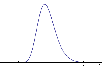
Suppose you have n random variables that have a log-normal(1, σ) distribution. Their product will have a log-normal(n, √n σ) distribution. As n increases, the distribution of the product becomes more skewed. Here is an example. The following graph shows the density of a log-normal(1, 0.2) distribution.

plot of log-normal(1, 0.2) density

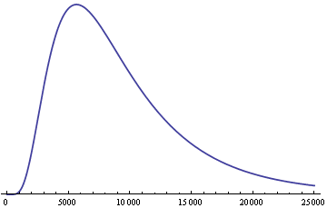
Here is the distribution of the product of nine independent copies of the above distribution, a log-normal(9, 0.6) distribution.

plot of log-normal(9, 0.6) density

So even though the original distribution is symmetric and concentrated near the middle, the product of nine independent copies has a long tail to the right.

Small advantages show up in the extremes
Variation in male and female Olympic performance: Part 1, Part 2
Evaluate people at their best or at their worst?

JavaScript: A picture is worth a thousand words

Posted on 28 September 2009 by John

Here’s a photo posted by David Walsh on Twitter on yesterday.

Related links:

How many trig functions are there?

Posted on 25 September 2009 by John

How many basic trigonometric functions are there? I will present the arguments for 1, 3, 6, and at least 12.

The calculator answer: 3

A typical calculator has three trig functions if it has any: sine, cosine, and tangent. The other three that you may see — cosecant, secant, and cotangent — are the reciprocals of sine, cosine, and tangent respectively. Calculator designers expect you to push the cosine key followed by the reciprocal key if you want a secant, for example.

The calculus textbook answer: 6

The most popular answer to the number of basic trig functions may be six. Unlike calculator designers, calculus textbook authors find the cosecant, secant, and cotangent functions sufficiently useful to justify their inclusion as first-class trig functions.

The historical answer: At least 12

There are at least six more trigonometric functions that at one time were considered worth naming. These are versine, haversine, coversine, hacoversine, exsecant, and excosecant. All of these can be expressed simply in terms of more familiar trig functions. For example, versine(θ) = 2 sin²(θ/2) = 1 – cos(θ) and exsecant(θ) = sec(θ) – 1.

Why so many functions? One of the primary applications of trigonometry historically was navigation, and certain commonly used navigational formulas are stated most simply in terms of these archaic function names. For example, the law of haversines. Modern readers might ask why not just simplify everything down to sines and cosines. But when you’re calculating by hand using tables, every named function takes appreciable effort to evaluate. If a table simply combines two common operations into one function, it may be worthwhile.

These function names have a simple pattern. The “ha-” prefix means “half,” just as in “ha’penny.” The “ex-” prefix means “subtract 1.” The “co-” prefix means what it always means. (More on that below.) The “ver-” prefix means 1 minus the co-function.

Pointless exercise: How many distinct functions could you come up with using every combination of prefixes? The order of prefixes might matter in some cases but not in others.

The minimalist answer: 1

The opposite of the historical answer would be the minimalist answer. We don’t need secants, cosecants, and cotangents because they’re just reciprocals of sines, cosines, and tangents. And we don’t even need tangent because tan(θ) = sin(θ)/cos(θ). So we’re down to sine and cosine, but then we don’t really need cosine because cos(θ) = sin(π/2 – θ).

Not many people remember that the “co” in cosine means “complement.” The cosine of an angle θ is the sine of the complementary angle π/2 – θ. The same relationship holds for secant and cosecant, tangent and cotangent, and even versine and coversine.

By the way, understanding this complementary relationship makes calculus rules easier to remember. Let foo(θ) be a function whose derivative is bar(θ). Then the chain rule says that the derivative of foo(π/2 – θ) is -bar(π/2 – θ). In other words, if the derivative of foo is bar, the derivative of cofoo is negative cobar. Substitute your favorite trig function for “foo.” Note also that the “co-” function of a “co-” function is the original function. For example, co-cosine is sine.

The consultant answer: It depends

The number of trig functions you want to name depends on your application. From a theoretical view point, there’s only one trig function: all trig functions are simple variations on sine. But from a practical view point, it’s worthwhile to create names like tan(θ) for the function sin(θ)/sin(π/2 – θ). And if you’re a navigator crossing an ocean with books of trig tables and no calculator, it’s worthwhile working with haversines etc.

Poverty versus squalor

Posted on 24 September 2009 by John

In his interview on EconTalk, Paul Graham made a distinction between poverty and squalor. He says that most poor people live like rich people, but with cheap imitations. A rich person might have something made of gold and a poor person might have the same thing except made of plastic. But the creative poor, such as the proverbial starving artist, live differently. They live in poverty but not in squalor. They achieve a pleasant lifestyle by not trying to imitate the rich.

For example, the wealthy have large beautiful houses. The poor have small and usually not-so-beautiful houses. The rich have new expensive cars and the poor have old cheap cars. But the starving artist might not have a house or a car. He or she might live in a converted warehouse with a few nice furnishings and ride a bicycle.

The point of his discussion of poverty was to make an analogy for small software companies. It makes no sense for a tiny start-up to try to be a scaled-down version of Microsoft. They need to have an entirely different strategy. They can be poor without living in squalor.

I don’t know what I think of Graham’s assertion that the poor live cheap imitations of the lifestyles of the rich. There’s probably some truth to it, though I’m not sure how much. And I’m not sure how much truth there is in the romantic image of the bohemian starving artist. But I agree that it makes no sense for a small company to be a miniature version of a huge corporation.

Feed the stars, milk the cows, and shoot the dogs

Posted on 23 September 2009 by John

The blog Confessions of a Community College Dean had a post on Monday entitled Cash Cows that talks candidly about the financial operations of a community college.

It’s a commonplace of for-profit management that units can be characterized in one of three ways: rising stars, cash cows, and dogs. The savvy manager is supposed to feed the stars, milk the cows, and shoot the dogs. … We milk the cows precisely so we don’t have to shoot the dogs.

The “cows” are the profitable courses and the “dogs” are the unprofitable courses. Popular belief has it that English classes are cash cows because they require fewer resources than, say, chemistry classes. However, this blog says that English classes only break even because they also have smaller classes. The real cash cows are the social sciences. The biggest dog is nursing. The profit from teaching history, for example, makes it possible to train nurses.

Software profitability in the middle

Posted on 22 September 2009 by John

Kent Beck made an interesting observation about the limits of open source software on FLOSS Weekly around one hour into the show. These aren’t his exact words, just my summary.

Big companies like IBM will contribute to big open source projects like Apache because doing so is in their economic interest. And hobbyists will write small applications and give them away. But who is going to write medium-sized software, projects big enough to be useful but not important enough to any one company to fund? That’s where commercial software thrives.

Kent Beck attributes this argument to Paul Davis.

Beck also talked about how he tried but couldn’t pay his bills developing open source software. The hosts were a little defensive and pointed out that many people have managed to earn money indirectly from open source software. Beck agreed but said that the indirect approach didn’t work for him. He said that he donates about 10% of his time to open source development (i.e. xUnit) but he makes his money by charging for his products and services.

Three views of the negative binomial distribution

Posted on 22 September 2009 by John

The negative binomial distribution is interesting because it illustrates a common progression of statistical thinking. My aim here is to tell a story, not to give details; the details are available here. The following gives a progression of three perspectives.

First view: Counting

The origin of the negative binomial is very concrete. It is unfortunate that the name makes the distribution seem more abstract than it is. (What could possibly be negative about a binomial distribution? Sounds like abstract nonsense.)

Suppose you have decided to practice basketball free throws. You’ve decided to practice until you have made 20 free throws. If your probability of making a single free throw is p, how many shots will you have to attempt before you make your goal of 20 successes? Obviously you’ll need at least 20 attempts, but you might need a lot more. What is the expected number of attempts you would need? What’s the probability that you’ll need more than 50 attempts? These questions could be answered by using a negative binomial distribution. A negative binomial probability distribution with parameters r and p gives the probabilities of various numbers of failures before the rth success when each attempt has probability of success p.

Second view: Cheap generalization

After writing down the probability mass function for the negative binomial distribution as described above, somebody noticed that the number r didn’t necessarily have to be an integer. The distribution was motivated by integer values of r, counting the number of failures before the rth success, but the resulting formula makes sense even when r is not an integer. It doesn’t make sense to wait for 2.87 successes; you can’t interpret the formula as counting events unless r is an integer, but the formula is still mathematically valid.

The probability mass function involves a binomial coefficient. These coefficients were first developed for integer arguments but later extended to real and even complex arguments. See these notes for definitions and these notes for how to calculate the general coefficients. The probability mass function can be written most compactly when one of the binomial coefficient has a negative argument. See page two of these notes for an explanation. There’s no intuitive explanation of the negative argument. It’s just a consequence of some algebra.

What’s the point in using non-integer values of r? Just because we can? No, there are practical reasons, and that leads to our third view.

Third view: Modeling overdispersion

Next we take the distribution above and forget where it came from. It was motivated by counting successes and failures, but now we forget about that and imagine the distribution falling from the sky in its general form described above. What properties does it have?

The negative binomial distribution turns out to have a very useful property. It can be seen as a generalization of the Poisson distribution. (See this distribution chart. Click on the dashed arrow between the negative binomial and Poisson boxes.)

The Poisson is the simplest distribution for modeling count data. It is in some sense a very natural distribution and it has nice theoretical properties. However, the Poisson distribution has one severe limitation: its variance is equal to its mean. There is no way to increase the variance without increasing the mean. Unfortunately, in many data sets the variance is larger than the mean. That’s where the negative binomial comes in. When modeling count data, first try the simplest thing that might work, the Poisson. If that doesn’t work, try the next simplest thing, negative binomial.

When viewing the negative binomial this way, a generalization of the Poisson, it helps to use a new parameterization. The parameters r and p are no longer directly important. For example, if we have empirical data with mean 20.1 and variance 34.7, we would naturally be interested in the negative binomial distribution with this mean and variance. We would like a parametrization that reflects more directly the mean and variance and one that makes the connection with the Poisson more transparent. That is indeed possible, and is described in these notes.

Update: Here’s a new post giving a fourth view of the negative binomial distribution — a continuous mixture of Poisson distributions. This view explains why the negative binomial is related to the Poisson and yet has greater variance.

Free alternative to Consolas font

Posted on 21 September 2009 by John

Consolas is my favorite monospace font. It’s a good programmer’s font because it exaggerates the differences between some characters that may easily be confused. It ships with Visual Studio and with many other Microsoft products. See this post for examples.

I recently found out about Inconsolata, a free font similar to Consolas. Inconsolata is part of the OFL font collection from SIL International.

Another interesting font from SIL is Andika, mentioned previously here. The Andika home page describes this font as follows.

Andika is a sans serif, Unicode-compliant font designed especially for literacy use, taking into account the needs of beginning readers. The focus is on clear, easy-to-perceive letterforms that will not be readily confused with one another.

Inverse Mercator projection

Posted on 21 September 2009 by John

In my earlier post on the Mercator projection, I derived the function h(φ) that maps latitude on the Earth to vertical height on a map. The inverse of this function turns out to hold a few surprises.

The height y corresponding to a positive latitude φ is given by

h(φ) = log( sec(φ) + tan(φ) ).

The inverse function, h^-1(y) = φ gives the latitude as a function of height. This function is called the “Gudermannian” after Christoph Gudermann and is abbreviated gd(y). Gudermann was the student of one famous mathematician, Karl Friedrich Gauss, and the teacher of another famous mathematician, Karl Weierstrass.

The Gudermannian function gd(y) can be reduced to familiar functions:

gd(y) = arctan( sinh(y) ) = 2 arctan( e^y ) – π/2.

That doesn’t look very promising. But here’s the interesting part: the function gd forms a bridge between hyperbolic trig functions and ordinary trig functions.

sin( gd(x) ) = tanh(x)
tan( gd(x) ) = sinh(x)
cos( gd(x) ) = sech(x)
sec( gd(x) ) = cosh(x)
csc( gd(x) ) = coth(x)
cot( gd(x) ) = csch(x)

By definition, gd(x) is an angle θ whose tangent is sinh(x).

In the figure, tan(θ) = sinh(x). Since cosh²(x) – sinh²(x) = 1, the hypotenuse of the triangle is cosh(x). The identities above follow directly from the figure. For example, sin(θ) = sinh(x) / cosh(x) = tanh(x).

Finally, it is easy to show that gd is the inverse of the Mercator scale function h:

h( gd(x) ) = log( sec( gd(x) ) + tan( gd(x) ) ) = log( cosh(x) + sinh(x) ) = log( e^x ) = x.

Month: September 2009