Parameters and percentiles

The doctor says 10% of patients respond within 30 days of treatment and 80% respond within 90 days of treatment. Now go turn that into a probability distribution. That’s a common task in Bayesian statistics, capturing expert opinion in a mathematical form to create a prior distribution.
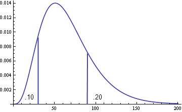
Graph of gamma density with 10th percentile at 30 and 80th percentile at 90

Things would be easier if you could ask subject matter experts to express their opinions in statistical terms. You could ask “If you were to represent your belief as a gamma distribution, what would the shape and scale parameters be?” But that’s ridiculous. Even if they understood the question, it’s unlikely they’d give an accurate answer. It’s easier to think in terms of percentiles.

Asking for mean and variance are not much better than asking for shape and scale, especially for a non-symmetric distribution such as a survival curve. Anyone who knows what variance is probably thinks about it in terms of a normal distribution. Asking for mean and variance encourages someone to think about a symmetric distribution.

So once you have specified a couple percentiles, such as the example this post started with, can you find parameters that meet these requirements? If you can’t meet both requirements, how close can you come to satisfying them? Does it depend on how far apart the percentiles are? The answers to these questions depend on the distribution family. Obviously you can’t satisfy two requirements with a one-parameter distribution in general. If you have two requirements and two parameters, at least it’s feasible that both can be satisfied.

If you have a random variable X whose distribution depends on two parameters, when can you find parameter values so that Prob(Xx1) = p1 and Prob(Xx2) = p2? For starters, if x1 is less than x2 then p1 must be less than p2. For example, the probability of a variable being less than 5 cannot be bigger than the probability of being less than 6. For some common distributions, the only requirement is this requirement that the x‘s and p‘s be in a consistent order.

For a location-scale family, such as the normal or Cauchy distributions, you can always find a location and scale parameter to satisfy two percentile conditions. In fact, there’s a simple expression for the parameters. The location parameter is given by

\frac{x_1 F^{-1}(p_2) - x_2 F^{-1}(p_1)}{F^{-1}(p_2) - F^{-1}(p_1)}

and the scale parameter is given by

\frac{x_2 - x_1}{F^{-1}(p_2) - F^{-1}(p_1)}

where F(x) is the CDF of the distribution representative with location 0 and scale 1.

The shape and scale parameters of a Weibull distribution can also be found in closed form. For a gamma distribution, parameters to satisfy the percentile requirements always exist. The parameters are easy to determine numerically but there is no simple expression for them.

For more details, see Determining distribution parameters from quantiles. See also the ParameterSolver software.

Update: I posted an article on CodeProject with Python code for computing the parameters described here.

Related posts

Universal time

Universal time (UTC) is the same as Greenwich Mean Time (GMT), give or take a second. It’s essentially the time in Greenwich, England except it ignores Daylight Savings Time.

The abbreviation UTC is an odd compromise. The French wanted to use the abbreviation TUC (temps universel coordonné) and the English wanted to use CUT (coordinated universal time). The compromise was UTC, which doesn’t actually abbreviate anything.

Sometimes a ‘Z’ is appended to a time to indicate it is expressed in UTC. The NATO phonetic alphabet code for ‘Z’ is ZULU, and so UTC is sometimes called “Zulu Time.”

It’s useful to know how your time zone relates to UTC. (You can look it up here.) For example, I live in the US Central time zone. Central Standard Time (CST) is UTC-6, i.e. we’re 6 hours behind Greenwich. Knowing your time relative to UTC makes international communication easier. It also helps you read computer time stamps since these almost always use UTC.

One of the advantages of UTC is that it avoids Daylight Savings Time. DST is surprisingly complicated when you look at it in detail. Some countries observe DST and some do not. Countries that do observe DST may begin and end DST on different dates, and those dates can change from year to year. And inside countries that observe DST some regions are exceptions. For example, the United States generally observes DST, but Arizona does not. Actually, it’s even more complicated: The Navajo Nation inside Arizona does observe DST.

Related posts

Statisticians take themselves too seriously

I suppose most people take themselves too seriously, but I’ve been thinking specifically about how statisticians take themselves too seriously.

The fundamental task of statistics is making decisions in the presence of uncertainty, and that’s hard. You have to make all kinds of simplifying assumptions and arbitrary choices to get anywhere. But after a while you lose sight of these decisions. Or you justify your decisions after the fact, making a virtue out of a necessity. After you’ve worked on a problem long enough, it’s nearly impossible to say “Of course, our whole way of thinking about this might have been wrong from the beginning.”

My concern is not so much “creative” statistics but rather uncreative statistics, rote application of established methods. Statistics is extremely conventional. But a procedure is not objective just because it is conventional.  An arbitrary choice made 80 years ago is still an arbitrary choice.

I’ve taken myself too seriously at times in regard to statistical matters; it’s easy to get caught up in your model. But I’m reminded of a talk I heard one time in which the speaker listed a number of embarrassing things that people used to believe. He was not making a smug comparison of how sophisticated we are now compared to our ignorant ancestors. Instead, his point was that we too may be mistaken. He exhorted everyone to look in a mirror and say “I may be wrong. I may be very, very wrong.”

Related posts

Engineering in the open

From Herbert Hoover, mining engineer and 31st President of the United States:

The great liability of the engineer compared to men of other professions is that his works are out in the open where all can see them. His acts, step by step, are in hard substance. He cannot bury his mistakes in the grave like the doctors. He cannot argue them into thin air or blame the judge like the lawyers. He cannot, like the architects, cover his failures with trees and vines. He cannot, like the politicians, screen his short-comings by blaming his opponents and hope the people will forget. The engineer simply cannot deny he did it. If his works do not work, he is damned.

Herbert Hoover photo

More engineering posts

Estimating reporting rates

Suppose the police department in your community reported an average of 10 burglaries per month. You could take that at face value and assume there are 10 burglaries per month. But maybe there are 20 burglaries a month but only half are reported.  How could you tell?

Here’s a similar problem.  Suppose you gave away an electronic book.  You stated that people are free to distribute it however they want, but that you’d appreciate feedback.  How could you estimate the number of people who have read the book?  If you get email from 100 readers, you know at least 100 people have read it, but maybe 10,000 people have read it and only 1% sent email.  How can you estimate the number of readers and the percentage who send email at the same time?

The key is the variability in the data.  You could never tell by looking at the average alone. If there were an average of 10 burglaries per month, the data would be less variable than if there were an average of 20 burglaries per month with only half reported.  Along the same lines, big variations in the amount of fan mail suggest that there may be many readers but few who send email.

The statistical problem is estimating the parameters (n, p) of a binomial distribution. The expected number of reported events is np where n is the total number of events and p is the probability that an event will be reported. Suppose one town has n1 actual burglaries with each burglary having a probability p1 of being reported. The other town has n2 burglaries with a probability p2 of being reported. If the expected number of reported burglaries are equal, then n1p1 = n2 p2 = r. The variance in the burglary reports from the two towns will be r(1 – p1) and r(1 – p2). If p1 is less than p2 there will be more variance in the data from the first city.

Estimating binomial parameters is complicated and I won’t give the details here.  If n were known, estimating p would be trivial. But when n and p are both unknown, this is a much harder problem. Still, there are ways to approach the problem.

Make something and sell it

I’ve run across a couple podcasts this week promoting the radical idea that you should sell what you make.

The latest Entrepreneurial Thought Leaders podcast features David Heineimeier Hansson’s talk Unlearn Your MBA which he gave to a room full of MBA students.

The latest Tech Nation podcast from IT Conversations is an interview with Jaron Lanier. Lanier is a virtual reality pioneer and the author of You Are Not A Gadget.

Both Hansson and Lanier have contributed to the “free” culture but both are also critical of it. Hansson says he has benefited greatly from open source software and make his Ruby on Rails framework open source as a way to contribute back to the open source community. But he is also scathingly critical of businesses that think they can make money by giving everything away.

Lanier was an early critic of intellectual property rights but has reversed his original position. He says he’s an empiricist and that data have convinced him he was dead wrong. He now says that the idea of giving away intellectual property as advertising bait is unsustainable and will have dire consequences.

Giving away content to make money indirectly works for some businesses. But it’s alarming that so many people believe that is the only rational or moral way to make money if you create intellectual property. Many people are saying things such as the following.

  • Musicians should give away their music and make money off concerts and T-shirts.
  • Authors should give away their books and make money on the lecture circuit.
  • Programmers should give away their software and make money from consulting.

There’s an anti-intellectual thread running through these arguments. It’s a materialistic way of thinking, valuing only tangible artifacts and not ideas. It’s OK for a potter to sell pots, but a musician should not sell music. It’s OK for teachers to make money by the hour for teaching, but they should not make money from writing books. It’s OK for programmers to sell their time as consultants, and maybe even to sell their time as a programmers, but they should not sell the products of their labor. It’s OK to sell physical objects or to sell time, but not to sell intellectual property.

Related post:

How to compute the soft maximum

The most obvious way to compute the soft maximum can easily fail due to overflow or underflow.

The soft maximum of x and y is defined by

g(x, y) = log( exp(x) + exp(y) ).

The most obvious way to turn the definition above into C code would be

double SoftMaximum(double x, double y)
{
    return log( exp(x) + exp(y) );
}

This works for some values of x and y, but fails if x or y is large. For example, if we use this to compute the soft maximum of 1000 and 200, the result is numerical infinity. The value of exp(1000) is too big to represent in a floating point number, so it is computed as infinity. exp(200) is finite, but the sum of an infinity and a finite number is infinity. Then the log function applied to infinity returns infinity.

We have the opposite problem if we try to compute the soft maximum of -1000 and -1200. In this computation exp(-1000) and exp(-1200) both underflow to zero, and the log function returns negative infinity for the logarithm of zero.

Fortunately it’s not hard to fix the function SoftMaximum to avoid overflow and underflow. Look what happens when we shift both arguments by a constant.

log( exp(xk) + exp(yk) ) = log( exp(x) + exp(y) ) – k.

This says

log( exp(x) + exp(y) ) = log( exp(xk) + exp(yk) ) + k

If we pick k to be the maximum of x and y, then one of the calls to exp has argument 0 (and so it returns 1) and the other has a negative argument. This means the follow code cannot overflow.

double SoftMaximum(double x, double y)
{
	double maximum = max(x, y);
	double minimum = min(x, y);
	return maximum + log( 1.0 + exp(minimum - maximum) );
}

The call to exp(minimum - maximum) could possibly underflow to zero, but in that case the code returns maximum. And in that case the return value is very accurate: if maximum is much larger than minimum, then the soft maximum is essentially equal to maximum.

The equation for the soft maximum implemented above has a few advantages in addition to avoiding overflow. It makes it clear that the soft maximum is always greater than the maximum. Also, it shows that the difference between the hard maximum and the soft maximum is controlled by the spread of the arguments. The soft maximum is nearest the hard maximum when the two arguments are very different and furthest from the hard maximum when the two arguments are equal.

Thanks to Andrew Dalke for suggesting the topic of this post by his comment.

Related links

Ten surprises from numerical linear algebra

Here are ten things about numerical linear algebra that you may find surprising if you’re not familiar with the field.

  1. Numerical linear algebra applies very advanced mathematics to solve problems that can be stated with high school mathematics.
  2. Practical applications often require solving enormous systems of equations, millions or even billions of variables.
  3. The heart of Google is an enormous linear algebra problem. PageRank is essentially an eigenvalue problem.
  4. The efficiency of solving very large systems of equations has benefited at least as much from advances in algorithms as from Moore’s law.
  5. Many practical problems — optimization, differential equations, signal processing, etc. — boil down to solving linear systems, even when the original problems are non-linear. Finite element software, for example, spends nearly all its time solving linear equations.
  6. A system of a million equations can sometimes be solved on an ordinary PC in under a millisecond, depending on the structure of the equations.
  7. Iterative methods, methods that in theory require an infinite number of steps to solve a problem, are often faster and more accurate than direct methods, methods that in theory produce an exact answer in a finite number of steps.

More applied linear algebra

Don’t invert that matrix

There is hardly ever a good reason to invert a matrix.

What do you do if you need to solve Ax = b where A is an n x n matrix? Isn’t the solution A-1 b? Yes, theoretically. But that doesn’t mean you need to actually find A-1. Solving the equation Ax = b is faster than finding A-1. Books might write the problem as x = A-1 b, but that doesn’t mean they expect you to calculate it that way.

What if you have to solve Ax = b for a lot of different b‘s? Surely then it’s worthwhile to find A-1. No. The first time you solve Ax = b, you factor A and save that factorization. Then when you solve for the next b, the answer comes much faster. (Factorization takes O(n3) operations. But once the matrix is factored, solving Ax = b takes only O(n2) operations. Suppose n = 1,000. This says that once you’ve solved Ax = b for one b, the equation can be solved again for a new b 1,000 times faster than the first one. Buy one get one free.)

What if, against advice, you’ve computed A-1. Now you might as well use it, right? No, you’re still better off solving Ax = b than multiplying by A-1, even if the computation of A-1 came for free. Solving the system is more numerically accurate than the performing the matrix multiplication.

It is common in applications to solve Ax = b even though there’s not enough memory to store A-1. For example, suppose n = 1,000,000 for the matrix A but A has a special sparse structure — say it’s banded — so that all but a few million entries of A are zero.  Then A can easily be stored in memory and Ax = b can be solved very quickly. But in general A-1 would be dense. That is, nearly all of the 1,000,000,000,000 entries of the matrix would be non-zero.  Storing A requires megabytes of memory, but storing A-1 would require terabytes of memory.

Related post: Applied linear algebra