Recognizing numbers

I was playing around with SymPy, a symbolic math package for Python, and ran across nsimplify. It takes a floating point number and tries to simplify it: as a fraction with a small denominator, square root of a small integer, an expression involving famous constants, etc.

For example, suppose some calculation returned 4.242640687119286 and you suspect there’s something special about that number. Here’s how you might test where it came from.

    >>> from sympy import *
    >>> nsimplify(4.242640687119286)
    3*sqrt(2)

Maybe you do a calculation numerically, find a simple expression for the result, and that suggests an analytical solution.

I think a more common application of nsimplify might be to help you remember half-forgotten formulas. For example, maybe you’re rusty on your trig identities, but you remember that cos(π/6) is something special.

    >>> nsimplify(cos(pi/6))
    sqrt(3)/2

Or to take a more advanced example, suppose that you vaguely remember that the gamma function takes on recognizable values at half integer values, but you don’t quite remember how. Maybe something involving π or e. You can suggest that nsimplify include expressions with π and e in its search.

    >>> nsimplify(gamma(3.5), constants=[pi, E])
    15*sqrt(pi)/8

You can also give nsimplify a tolerance, asking it to find a simple representation within a neighborhood of the number. For example, here’s a way to find approximations to π.

    >>> nsimplify(pi, tolerance=1e-5)
    355/113

With a wider tolerance, it will return a simpler approximation.

    >>> nsimplify(pi, tolerance=1e-2)
    22/7

Finally, here’s higher precision approximation to π that isn’t exactly simple:

    >>> nsimplify(pi, tolerance=1e-7)
    exp(141/895 + sqrt(780631)/895)

More sides or more dice?

My previous post looked at rolling 5 six-sided dice as an approximation of a normal distribution. If you wanted a better approximation, you could roll dice with more sides, or you could roll more dice. Which helps more?

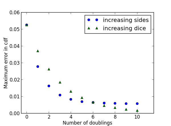
Whether you double the number of sides per die or double the number of dice, you have the same total number of spots possible. But which approach helps more? Here’s a plot.

We start with 5 six-sided dice and either double the number of sides per die (the blue dots) or double the number of dice (the green triangles). When the number of sides n gets big, it’s easier to think of a spinner with n equally likely stopping points than an n-sided die.

At first, increasing the number of sides per die reduces the maximum error more than the same increase in the number of dice. But after doubling six times, i.e. increasing by a factor of 64, both approaches have the same error. But further increasing the number of sides per die makes little difference, while continuing to increase the number of dice decreases the error.

The long-term advantage goes to increasing the number of dice. By the central limit theorem, the error will approach zero as the number of dice increases. But with a fixed number of dice, increasing the number of sides only makes each die a better approximation to a uniform distribution. In the limit, your sum approximates a normal distribution no better or worse than the sum of five uniform distributions.

But in the near term, increasing the number of sides helps more than adding more dice. The central limit theorem may guide you to the right answer eventually, but it might mislead you at first.

Rolling dice for normal samples: Python version

A handful of dice can make a decent normal random number generator, good enough for classroom demonstrations. I wrote about this a while ago.

My original post included Mathematica code for calculating how close to normal the distribution of the sum of the dice is. Here I’d like to redo the code in Python to show how to do the same calculations using SymPy. [Update: I’ll also give a solution that does not use SymPy and that scales much better.]

If you roll five dice and add up the spots, the probability of getting a sum of k is the coefficient of xk in the expansion of

(x + x2 + x3 + x4 + x5 + x6)5 / 65.

Here’s code to find the probabilities by expanding the polynomial and taking coefficients.

    from sympy import Symbol

    sides = 6
    dice = 5
    rolls = range( dice*sides + 1 )

    # Tell SymPy that we want to use x as a symbol, not a number
    x = Symbol('x')

    # p(x) = (x + x^2 + ... + x^m)^n
    # where m = number of sides per die
    # and n = number of dice
    p = sum( x**i for i in range(1, sides + 1) )**dice

    # Extract the coefficients of p(x) and divide by sides**dice
    pmf = [sides**(-dice) * p.expand().coeff(x, i) for i in rolls]

If you’d like to compare the CDF of the dice sum to a normal CDF you could add this.

    from scipy import array, sqrt
    from scipy.stats import norm

    cdf = array(pmf).cumsum()

    # Normal CDF for comparison
    mean = 0.5*(sides + 1)*dice
    variance = dice*(sides**2 -1)/12.0
    temp = [norm.cdf(i, mean, sqrt(variance)) for i in roles]
    norm_cdf = array(temp)

    diff = abs(cdf - norm_cdf)
    # Print the maximum error and where it occurs
    print diff.max(), diff.argmax()

Question: Now suppose you want a better approximation to a normal distribution. Would it be better to increase the number of dice or the number of sides per dice? For example, would you be better off with 10 six-sided dice or 5 twelve-sided dice? Think about it before reading the solution.

Update: The SymPy code does not scale well. When I tried the code with 50 six-sided dice, it ran out of memory. Based on Andre’s comment, I rewrote the code using polypow. SymPy offers much more symbolic calculation functionality than NumPy, but in this case NumPy contains all we need. It is much faster and it doesn’t run out of memory.

    from numpy.polynomial.polynomial import polypow
    from numpy import ones

    sides = 6
    dice = 100

    # Create an array of polynomial coefficients for
    # x + x^2 + ... + x^sides
    p = ones(sides + 1)
    p[0] = 0

    # Extract the coefficients of p(x)**dice and divide by sides**dice
    pmf = sides**(-dice) * polypow(p, dice)
    cdf = pmf.cumsum()

That solution works for up to 398 dice. What’s up with that? With 399 dice, the largest polynomial coefficient overflows. If we divide by the number of dice before raising the polynomial to the power dice, the code becomes a little simpler and scales further.

    p = ones(sides + 1)
    p[0] = 0
    p /= sides
    pmf = polypow(p, dice)
    cdf = pmf.cumsum()

I tried this last approach on 10,000 dice with no problem.

2,000th post

This is my 2,000th blog post. I’ve been blogging for a little over five years, writing around a post a day. Thank you all for reading, commenting, sharing, and generally being so encouraging. This post will just be a few brief updates.

Blog upgrade

I upgraded my blogging software and changed the theme a few weeks ago. The new theme is supposed to be more mobile-friendly. There were a few little problems with the upgrade. I think I’ve fixed everything by now, though I’d still like to make a few changes here and there. If you see any problems or have any suggestions, please let me know.

Consulting

Going out on my own has been a blast. I’ve got a few projects going on now and more on the horizon. Really interesting work. As you’d expect if you’ve read this blog for a while, the work has been a mixture of math, stats, computing, and writing. I may be hiring a couple people part-time to help me out.

Google Reader

If you’ve subscribed to this blog through Google Reader, remember that Google is going to turn it off July 1. There are many other RSS readers out there. I list a few options here. My impression is that a lot of the people are moving to Feedly or NewsBlur.

Travel

I plan to visit Tuscaloosa, San Francisco, and Austin in the next few weeks. Let me know if you’re in one of these areas and would like to get together.

Hacking debt

The term technical debt describes the accumulated effect of short term decisions in a software development process. In order to meet a deadline, for example, a project will take shortcuts, developing code in a way that’s not best for future maintainability but that saves time immediately. Once the pressure is off, hopefully, the team goes back and repays the technical debt by refactoring.

I’d like to propose hacking debt to describe a person who has been focused on “real work” for so long that he or she hasn’t spent enough time playing around, making useless stuff for the fun of it. Some portion of a career should be devoted to hacking. Not 100%, but not 0% either. Without some time spent exploring and having fun, people become less effective and eventually burn out.

Related posts

For hacking financial debt, see this.

Bad normal approximation

Sometimes you can approximate a binomial distribution with a normal distribution. Under the right conditions, a Binomial(n, p) has approximately the distribution of a normal with the same mean and variance, i.e. mean np and variance np(1-p). The approximation works best when n is large and p is near 1/2.

This afternoon I was reading a paper that used a normal approximation to a binomial when n was around 10 and p around 0.001.  The relative error was enormous. The paper used the approximation to find an analytical expression for something else and the error propagated.

A common rule of thumb is that the normal approximation works well when np > 5 and n(1-p) > 5.  This says that the closer p is to 0 or 1, the larger n needs to be. In this case p was very small, but n was not large enough to compensate since np was on the order of 0.01, far less than 5.

Another rule of thumb is that normal approximations in general hold well near the center of the distribution but not in the tails. In particular the relative error in the tails can be unbounded. This paper was looking out toward the tails, and relative error mattered.

For more details, see these notes on the normal approximation to the binomial.

Why j for imaginary unit?

Electrical engineers use j for the square root of -1 while nearly everyone else uses i. The usual explanation is that EE’s do this because they use i for current. But here’s one advantage to using j that has nothing to do with electrical engineering.

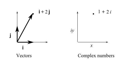
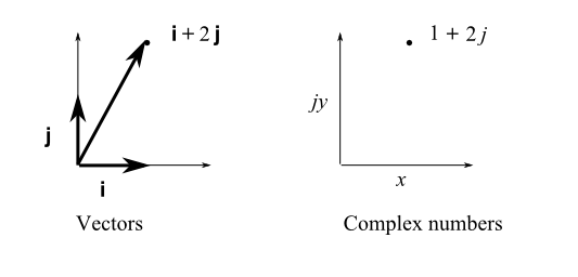
The symbols i, j, and k are used for unit vectors in the directions of the x, y, and z axes respectively. That means that “i” has two different meanings in the real plane, depending on whether you think of it as the vector space spanned by i and j or as complex numbers. But if you use j to represent the imaginary unit, its meaning does not change. Either way it points along the y axis.

Said another way, bold face i and italic i point in different directions But bold face j and italic j both point in the same direction.

Here’s what moving from vectors to complex numbers looks like in math notation:

And here’s what it looks like in electrical engineering notation:

I don’t expect math notation to change, nor would I want it to. I’m happy with i. But using j might make moving between vectors and complex numbers a little easier.

Related: Applied complex analysis

Quotation and endorsement

I like sharing quotes on Twitter. Occasionally a quote will provoke an angry reaction, not to the content of the quote but to the source. Sometimes people will even acknowledge that they agree with the quote, but are dismayed that I would quote such a despicable person.

This morning I was reading Norman Geisler’s book on Thomas Aquinas and these lines reminded me of the brouhaha over quotes and sources.

No, I do not agree with everything he [Aquinas] ever wrote. On the other hand, neither do I agree with everything I ever wrote.

I’d say along with Geisler that if I could only quote people I completely agreed with, I could not even quote myself.

Geisler goes on to say

But seven hundred years from now no one will even recognize my name, while Aquinas’ works will still be used with great profit.

I feel the same way about many of the people I quote. I remember catching flak for quoting Martin Luther. I’ve already forgotten the critic’s name, and he’s probably forgotten mine, but people will still be reading Luther in another five hundred years.

Moments of mixtures

I needed to compute the higher moments of a mixture distribution for a project I’m working on. I’m writing up the code here in case anyone else finds this useful. (And in case I’ll find it useful in the future.) I’ll include the central moments first. From there it’s easy to compute skewness and kurtosis.

Suppose X is a mixture of n random variables Xi with weights wi, non-negative numbers adding to 1. Then the jth central moment of X is given by

E[(X - \mu)^j] = \sum_{i=1}^n \sum_{k=0}^j {j \choose k} (\mu_i - \mu)^{j-k} w_i E[(X_i- \mu_i)^k]

where μi is the mean of Xi.

In my particular application, I’m interested in a mixture of normals and so the code below computes the moments for a mixture of normals. It could easily be modified for other distributions.

from scipy.misc import factorialk, comb

def mixture_central_moment(mixture, moment):

    '''Compute the higher moments of a mixture of normal rvs.
    mixture is a list of (mu, sigma, weight) triples.
    moment is the central moment to compute.'''

    mix_mean = sum( w*m for (m, s, w) in mixture )

    mixture_moment = 0.0
    for triple in mixture:
        mu, sigma, weight = triple
        for k in range(moment+1):
            prod = comb(moment, k) * (mu-mix_mean)**(moment-k)
            prod *= weight*normal_central_moment(sigma, k)
            mixture_moment += prod

    return mixture_moment

def normal_central_moment(sigma, moment):

    '''Central moments of a normal distribution'''

    if moment % 2 == 1:
        return 0.0
    else:
        # If Z is a std normal and n is even, E(Z^n) == (n-1)!!
        # So E (sigma Z)^n = sigma^n (n-1)!!
        return sigma**moment * factorialk(moment-1, 2)

Once we have code for central moments, it’s simple to add code for computing skewness and kurtosis.

def mixture_skew(mixture):

    variance = mixture_central_moment(mixture, 2)
    third = mixture_central_moment(mixture, 3)
    return third / variance**(1.5)

def mixture_kurtosis(mixture):

    variance = mixture_central_moment(mixture, 2)
    fourth = mixture_central_moment(mixture, 4)
    return fourth / variance**2 - 3.0

Here’s an example of how the code might be used.

# Test on a mixture of 30% Normal(-2, 1) and 70% Normal(1, 3)
mixture = [(-2, 1, 0.3), (1, 3, 0.7)]

print "Skewness = ", mixture_skew(mixture)
print "Kurtosis = ", mixture_kurtosis(mixture)

Related post: General formula for normal moments