Solving hard problems

We help companies solve hard problems in mathematics, statistics, and computing. Let’s explore how we might work together.

Jaccard index and jazz albums

Posted on 26 July 2023 by John

Miles Davis Kind of Blue album cover

Jaccard index is a way of measuring the similarity of sets. The Jaccard index, or Jaccard similarity coefficient, of two sets A and B is the number of elements in their intersection, A ∩ B, divided by the number of elements in their union, A ∪ B.

$J(A, B) = \frac{|A \cap B|}{|A \cup B|}$

Jaccard similarity is a robust way to compare things in machine learning, say in clustering algorithms, less sensitive to outliers than other similarity measures such as cosine similarity.

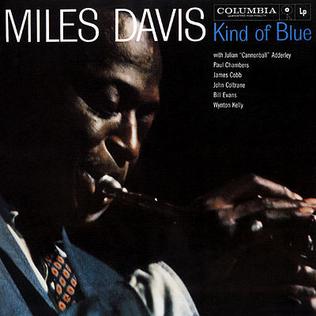
Miles Davis Albums

Here we’ll illustrate Jaccard similarity by looking at the personnel on albums by Miles Davis. Specifically, which pair of albums had more similar personnel: Kind of Blue and Round About Midnight, or Bitches Brew and In a Silent Way?

There were four musicians who played on both Kind of Blue and Round About Midnight: Miles Davis, Cannonball Adderly, John Coltrane, and Paul Chambers.

There were six musicians who played on both Bitches Brew and In a Silent Way: Miles Davis, Wayne Shorter, Chick Corea, Dave Holland, and John McLaughlin, Joe Zawinul.

The latter pair of albums had more personnel in common, but they also had more personnel in total.

There were 9 musicians who performed on either Kind of Blue or Round About Midnight. Since 4 played on both albums, the Jaccard index comparing the personnel on the two albums is 4/9.

In a Silent Way and especially Bitches Brew used more musicians. A total of 17 musicians performed on one of these albums, including 6 who were on both. So the Jaccard index is 6/17.

Jaccard distance

Jaccard distance is the complement of Jaccard similarity, i.e.

In our example, the Jaccard distance between Kind of Blue and Round About Midnight is 1 − 4/9 = 0.555. The Jaccard distance between Bitches Brew and In a Silent Way is 1 − 6/17 = 0.647.

Jaccard distance really is a distance. It is clearly a symmetric function of its arguments, unlike Kulback-Liebler divergence, which is not.

The difficulty in establishing that Jaccard distance is a distance function, i.e. a metric, is the triangle inequality. The triangle inequality does hold, though this is not simple to prove.

Trying NLP on Middle English

Posted on 25 July 2023 by John

It’s not fair to evaluate NLP software on a language it wasn’t designed to process, but I wanted to try it anyway.

The models in the spaCy software library were trained on modern English text and not on Middle English. Nevertheless, spaCy does a pretty good job of parsing Chaucer’s Canterbury Tales, written over 600 years ago. I used the model en_core_web_lg in my little experiment below.

The text I used comes from the prologue:

From every shires ende
of Engelond to Caunterbury they wende
the hooly blisful martir for to seke
that hem hath holpen
whan that they were seeke.

The software correctly identifies, for example, wende (went) and seke (seak) as verbs, and seeke (sick) as an adjective. Overall it does a pretty good job. I imagine it would do worse on Middle English text that differed more from Modern English usage, but so would a contemporary human who doesn’t know Middle English.

Extending harmonic numbers

Posted on 25 July 2023 by John

For a positive integer n, the nth harmonic number is defined to be the sum of the reciprocals of the first n positive integers:

$H_n = 1 + \frac{1}{2} + \frac{1}{3} + \cdots + \frac{1}{n}$

How might we extend this definition so that n does not have to be a positive integer?

First approach

One way to extend harmonic numbers is as follows. Start with the equation

$(t - 1)(t^{n-1} + t^{n-2} + t^{n-3} + \cdots + 1) = t^n - 1$

Then

$\frac{t^n - 1}{t-1} = t^{n-1} + t^{n-2} + t^{n-3} + \cdots + 1$

Integrate both sides from 0 to 1.

$\int_0^1\frac{t^n - 1}{t-1} \,dt = \frac{1}{n} + \frac{1}{n-1} + \frac{1}{n-2} + \cdots + 1 = H_n$

So when x is an integer,

$H_x = \int_0^1\frac{t^x - 1}{t-1} \,dt$

is a theorem. When x is not an integer, we take this as a definition.

Second approach

Another approach is to start with the identity

$\Gamma(x+1) = x\, \Gamma(x)$

then take the logarithm and derivative of both sides. This gives

$\psi(x+1) = \frac{1}{x} + \psi(x)$

where the digamma function ψ is defined to be the derivative of the log of the gamma function.

If x is an integer and we apply the identity above repeatedly we get

$\psi(n+1) = H_n + \psi(1) = H_n - \gamma$

where γ is Euler’s constant. Then we can define

$H_x = \psi(x + 1) + \gamma$

for general values of x.

Are they equal?

We’ve shown two ways of extending the harmonic numbers. Are these two different extensions or are they equal? They are in fact equal, which follows from equation 12.16 in Whittaker and Watson, citing a theorem of Legendre.

Taking either approach as our definition we could, for example, compute the πth harmonic number (1.87274) or even the ith harmonic number (0.671866 + 1.07667i).

An addition rule

The digamma function satisfies an addition rule

$\psi(2z) = \frac{1}{2} \left( \psi(z) + \psi\left(z + \frac{1}{2}\right)\right) + \log 2$

which can be proved by taking the logarithm and derivative of Gauss’s multiplication rule for the gamma function.

Let z = x + 1/2 and add γ to both sizes. This shows that harmonic numbers satisfy the addition rule

$H_{2x} = \frac{1}{2}\left( H_{x-1/2} + H_x \right) + \log 2$

A note on Zipf’s law

Posted on 25 July 2023 by John

Very often when a number is large, and we don’t know or care exactly how large it is, we can model it as infinite. This may make no practical difference and can make calculations much easier. I give several examples of this in the article Infinite is easier than big.

When you run across a statement that something is infinite, you can often mentally replace “infinite” with “big, but so big that it doesn’t matter exactly how big it is.” Conversely, the term “finite” in applied mathematics means “limited in a way that matters.”

But when we say something does or does not matter, there’s some implicit context. It does or does not matter for some purpose. We can get into trouble when we’re unclear of that context or when we shift contexts without realizing it.

Zipf’s law

Zipf’s law came up a couple days ago in a post looking at rare Chinese characters. That post resolves a sort of paradox, that rare characters come up fairly often. Each of these rare characters is very unlikely to occur in a document, and yet collectively its likely that some of them will be necessary.

In some contexts we can consider the number of Chinese characters or English words to be infinite. If you want to learn English by first learning the meaning of every English word, you will never get around to using English. The number of words is infinite in the sense that you will never get to the end.

Zipf’s law says that the frequency of the nth word in a language is proportional to n^−s. This is of course an approximation, but a surprisingly accurate approximation for such a simple statement.

Infinite N?

The Zipf probability distribution depends on two parameters: the exponent s and the number of words N. Since the number of words in any spoken language is large, and its impossible to say exactly how large it is, can we assume N = ∞? This seems like exactly the what we were talking about at the top of this article.

Whether it is possible to model N as infinite depends on s. The value of s that models word frequency in many languages is close to 1. The plot below illustrates Zipf’s law for the text of Wikipedia in many different languages. In each case, the slope on the log-log plot is approximately 1, i.e. s ≈ 1.

When s = 1, we don’t have a probability distribution because the sum of 1/n from 1 to ∞ diverges. And so no, we cannot assume N = ∞.

Now you may object that all we have to do is set s to be slightly larger than 1. If s = 1.0000001, then the sum of n^−s converges. Problem solved. But not really.

When s = 1 the series diverges, but when s is slightly larger than 1 the sum is very large. Practically speaking this assigns too much probability to rare words.

If s = 2, for example, one could set N = ∞. The Zipf distribution with s = 2 may be useful for modeling some things, but not for modeling word frequency.

Zipf’s law applied to word frequency is an interesting example of a model that contains a large N, and although it doesn’t matter exactly how large N is, it matters that N is finite. In the earlier article, I used the estimate that Chinese has 50,000 characters. If I had estimated 60,000 characters the conclusion of the article would not have been too different. But assuming an infinite number of characters would result in substantially overestimating the frequency of rare words.

Image above by Sergio Jimenez, CC BY-SA 4.0, via Wikimedia Commons

Natural language processing and unnatural text

Posted on 24 July 2023 by John

I recently evaluated two software applications designed to find PII (personally identifiable information) in free text using natural language processing. Both failed badly, passing over obvious examples of PII. By contrast, I also tried natural language processing software on a nonsensical poem, it the software did quite well.

Doctor’s notes

It occurred to me later that the software packages to search for PII probably assume “natural language” has the form of fluent prose, not choppy notes by physicians. The notes that I tested did not consist of complete sentences marked up with grammatically correct punctuation. The text may have been transcribed from audio.

Some software packages deidentify medical notes better than others. I’ve seen some work well and some work poorly. I suspect the former were written specifically for their purpose and the latter were more generic.

Jabberwocky

I also tried NLP software on Lewis Carroll’s poem Jabberwocky. It too is unnatural language, but in a different sense.

Jabberwocky uses nonsense words that Carroll invented for the poem, but otherwise it is grammatically correct. The poem is standard English at the level of structure, though not at the level of words. It is the opposite of medical notes that are standard English at the word level (albeit with a high density of technical terms), but not at a structural level.

I used the spaCy natural language processing library on a couple stanzas from Lewis’ poem.

“Beware the Jabberwock, my son!
The jaws that bite, the claws that catch!
Beware the Jubjub bird, and shun
The frumious Bandersnatch!”

He took his vorpal sword in hand;
Long time the manxome foe he sought—
So rested he by the Tumtum tree
And stood awhile in thought.

I fed the lines into spaCy and asked it to diagram the lines, indicating parts of speech and dependencies. The software did a good job of inferring the use of even the nonsense words. I gave the software one line at a time rather than a stanza at a time because the latter results in diagrams that are awkwardly wide, too wide to display here. (The spaCy visualization software has a “compact” option, but this option does not make the visualizations much more compact.)

Here are the visualizations of the lines.

And here is the Python code I used to create the diagrams above.

    import spacy
    from spacy import displacy
    from pathlib import Path
    
    nlp = spacy.load("en_core_web_sm")
        
    lines = [
        "Beware the Jabberwock, my son!",
        "The jaws that bite, the claws that catch!",
        "Beware the Jubjub bird",
        "Shun the frumious Bandersnatch!",
        "He took his vorpal sword in hand.",
        "Long time the manxome foe he sought",
        "So rested he by the Tumtum tree",
        "And stood awhile in thought."
    ]
    
    for line in lines:
        doc = nlp(line)
        svg = displacy.render(doc, style="dep", jupyter=False)    
        file_name = '-'.join([w.text for w in doc if not w.is_punct]) + ".svg"
        output_path = Path(file_name)
        output_path.open("w", encoding="utf-8").write(svg)

How rare is it to encounter a rare word?

Posted on 23 July 2023 by John

biáng

I recently ran across a paper on typesetting rare Chinese characters. From the abstract:

Written Chinese has tens of thousands of characters. But most available fonts contain only around 6 to 12 thousand common characters that can meet the needs of everyday users. However, in publications and information exchange in many professional fields, a number of rare characters that are not in common fonts are needed in each document.

There’s sort of a paradox here: the author is saying it’s common to need rare words. Aren’t rare words, you know, rare? Of course they are, but the chances of needing some rare word, not just a particular rare word, can be large, particularly in lengthy documents.

This post gives a sort of back-of-the-envelope calculation to justify the preceding paragraph.

Word frequencies often approximately follow Zipf’s law, where the frequency of the nth most common word is proportional to n raised to some negative power s. I’ve seen estimates that there are around N = 50,000 characters in Chinese, but that 1,000 characters make up about 90% of usage. This would correspond to a value of s around 1.25.

In practice, Zipf’s law, like all power laws, fits better over some parts of its range than others. We’re making a simplifying assumption by applying Zipf’s law to the entire vocabulary of Chinese, but this post isn’t trying to precisely model Chinese character frequency, only to show that the statement quoted above is plausible.

With our Zipf’s law model, the 10,000th most common character in Chinese would appear about 2 times in a million characters. But the frequency of all the words from the 10,000th most common to the 50,000th most common would be about 0.03.

So if we list all characters in order of frequency and call everything after the 10,000th position on the list rare, the combined frequency of all rare words is quite high, about 3%. To put it another way, a document of 1,000 words would likely contain around 30 rare words, according to the simplified model presented here.

[1] The Chinese character at the top of the post comes from here. According to the source, “The Chinese character ‘biáng’ used to represent Biang Biang noodles, is one of the most complex and rare Chinese characters. It has 56 strokes and cannot be found in modern dictionaries or entered into computers.”

How an LLM might leak medical data

Posted on 23 July 2023 by John

Machine learning models occasionally memorize training data. Under the right prompt, a model could return portions of the training data verbatim.

If a large language model is trained on deidentified medical data, along with data that overlaps with the medical data, it could potentially leak details of a person’s medical history. I’m not saying that any particular LLM does leak data, but it’s something to watch out for if you are training an LLM.

One way to try to create a data leak would be to prompt the LLM with the data you have and see whether it will fill in more. For example, I asked Bing AI

Tell me about a man from Arkansas with ICD-10 code C50.921.

It came back with the following.

… Once upon a time, there was a man named John who lived in Arkansas. John was a hardworking man who loved spending time with his family and friends. One day, John noticed a lump in his right breast. He went to the doctor and was diagnosed with malignant neoplasm of unspecified site of the right male breast, classified under the ICD-10 code C50.921. …

I chose this diagnosis code because male breast cancer is extremely rare, and so the risk of reidentification is higher than for a more common diagnosis.

The model filled in the detail that the man’s name is John. This is not at all suspicious since John is the one of the most common male names in history. If the man’s name had been Vivek, there would be more cause to suspect the model is telling us about a real man name Vivek, though of course that could be a randomly chosen male name.

If a neural network were training on deidentified medical data, it could link fields together. If the story above had said “John, aged 42, …” the age might have been pulled from an actual patient record.

If the data the network was trained on was deidentified well, even leaking data verbatim should not create more than a very small risk of identification. However, if the data contained tokens linking the records to publicly available information, such as real estate records—this happens—then our hypothetical LLM might reveal more personal details that could be used to narrow down whose data is being leaked.

V-statistics

Posted on 19 July 2023 by John

A few days ago I wrote about U-statistics, statistics which can be expressed as the average of a symmetric function over all combinations of elements of a set. V-statistics can be written as an average of over all products of elements of a set.

Let S be a statistical sample of size n and let h be a symmetric function of r elements. The average of h over all subsets of S with r elements is a U-statistic. The average of h over the Cartesian product of S with itself r times

$\underbrace{S \times S \times \cdots \times S}_{n \text{ times}}$

is a V-statistic.

As in the previous post, let h(x, y) = (x − y)²/2. We can illustrate the V-statistic associated with h with Python code as before.

    import numpy as np
    from itertools import product

    def var(xs):
        n = len(xs)
        h = lambda x, y: (x - y)**2/2
        return sum(h(*c) for c in product(xs, repeat=2)) / n**2

    xs = np.array([2, 3, 5, 7, 11])
    print(np.var(xs))
    print(var(xs))

This time, however, we iterate over product rather than over combinations. Note also that at the bottom of the code we print

   np.var(xs)

rather than

   np.var(xs, ddof=1)

This means our code here is computing the population variance, not the sample variance. We could make this more explicit by supplying the default value of ddof.

   np.var(xs, ddof=0)

The point of V-statistics is not to calculate them as above, but that they could be calculated as above. Knowing that a statistic is an average of a symmetric function is theoretically advantageous, but computing a statistic this way would be inefficient.

U-statistics are averages of a function h over all subsamples of S of size r without replacement. V-statistics are averages of h over all subsamples of size r with replacement. The difference between sampling with or without replacement goes away as n increases, and so V-statistics have the same asymptotic properties as U-statistics.

Filtering on how words are being used

Posted on 18 July 2023 by John

Yesterday I wrote about how you could use the spaCy Python library to find proper nouns in a document. Now suppose you want to refine this and find proper nouns that are the subjects of sentences or proper nouns that are direct objects.

This post was motivated by a project in which I needed to pull out company names from a large amount of text, and it was important to know how the company name was being used.

Dependency labels

Tokens in spaCy have a dependency label attribute dep (or dep_ for its string representation). Dependency labels tell you how a word is being used. For example, dobj tells you the word is being used as a direct object, and nsubj tells you its being used as a nominal subject.

In yesterday’s post the line

    if tok.pos_ == "PROPN":
        print(tok)

filtered tokens to look for proper nouns. We could modify the script to also tell us how the proper nouns are being used by printing tok.dep_.

There are three proper nouns in the opening paragraph of Moby Dick: Ishmael, November, and Cato.

Call me Ishmael. … whenever it is a damp, drizzly November in my soul … With a philosophical flourish Cato throws himself upon his sword …

If we run

    if tok.pos_ == "PROPN":
        print(tok, tok.dep_)

on the first paragraph we get

    Ishmael oprd
    November attr
    Cato nsubj

but it’s not obvious what the output means. If we wrap tok.dep_ with spacy.explain we get a more verbose explanation.

    Ishmael object predicate
    November attribute
    Cato nominal subject

Pulling out subjects

Now suppose we wanted to pull out words that are subjects. We could filter on tok.dep_ == "nsubj" but there are more kinds of subjects than just nominal subjects. There are six kinds of subjects:

nsubj: nominal subject
nsubjpass: nominal passive subject
csubj: clausal subject
csubjpass: clausal passive subject
agent: agent
expl: expletive

Finding the range of possible values for dependency labels takes some digging. I don’t believe it’s in the spaCy documentation per se, but if you’re persistent you’ll find a link this list or the paper it came from.

Forever chemicals and blood donation

Posted on 18 July 2023 by John

I saw a headline saying that donating blood lowers the level of forever chemicals in your body. This post will give a back-of-the-envelope calculation to show that this idea is plausible.

Suppose there are chemicals in your bloodstream that do not break down and that your body will not filter out. Suppose you have about 5 liters of blood and you donate 500ml of blood at a time, 10% of your total blood volume.

Presumably the blood you donate has the same proportion of forever chemicals as the blood you keep, so you lose 10% of your forever chemicals in a blood donation.

Assume you don’t absorb more forever chemicals after you start donating blood, and your body replaces the donated blood with new blood free of forever chemicals.

The quantity of forever chemicals in your blood after n donations is 0.9ⁿ times the original amount. How many donations would it take to reduce your level of forever chemicals by half?

We need to solve

0.9ⁿ = 0.5.

Taking logs we find

n = log(0.5)/log(0.9) = 6.58.

So after 7 donations, you should have reduced the level of forever chemicals in your blood by about a half. Assuming you donate every 8 weeks, this would take a little over a year.

This is just a simplistic calculation. The result could be inaccurate or even entirely incorrect for any number of reasons. But it does show that the idea that blood donation lowers forever chemical levels is plausible.

Solving hard problems

Jaccard index and jazz albums

Miles Davis Albums

Jaccard distance

Trying NLP on Middle English

Related posts

Extending harmonic numbers

First approach

Second approach

Are they equal?

An addition rule

Related posts

A note on Zipf’s law

Zipf’s law

Infinite N?

Related posts

Natural language processing and unnatural text

Doctor’s notes

Jabberwocky

Related posts

How rare is it to encounter a rare word?

Related posts

How an LLM might leak medical data

Related posts

V-statistics

Related posts

Filtering on how words are being used

Dependency labels

Pulling out subjects

Forever chemicals and blood donation