Fourier, Gauss, and Heisenberg

Posted on 7 June 2021 by John

Several weeks ago I wrote about the Fourier uncertainty principle which gives a lower bound on the product of the variance of a function f and the variance of its Fourier transform. This post expands on the earlier post by quoting some results from a recent paper [1].

Gaussian density

The earlier post said that the inequality in the Fourier uncertainty principle is exact when f is proportional to a Gaussian probability density. G. H. Hardy proved this result in 1933 in the form of the following theorem.

Let f be a square-integrable function on the real line and assume f and its Fourier transform satisfy the following bounds

$\begin{align*} |f(x)| \leq& \,C \exp(-a|x|^2) \\ |\hat{f}(\xi)| \leq& \,C \exp(-b|\xi|^2\,) \\ \end{align*}$

for some constant C. Then if ab > 1/4, then f = 0. And if ab = 1/4, f(x) = c exp(−ax²) for some constant c.

Let’s translate this into probability terms by setting

$\begin{align*} a =& \,\frac{1}{2\sigma^2} \\ b =& \,\frac{1}{2\tau^2} \end{align*}$

Now Hardy’s theorem says that if f is bounded by a multiple of a Gaussian density with variance σ² and its Fourier transform is bounded by a multiple of a Gaussian density with variance τ², then the product of the two variances is no greater than 1. And if the product of the variances equals 1, then f is a multiple of a Gaussian density with variance σ².

Heisenberg uncertainty

Theorem 3 in [1] says that if u(t, x) is a solution to the free Schrödinger’s equation

$\partial_t u = i \Delta u$

then u at different points in time satisfies a theorem similar to Hardy’s theorem. In fact, the authors show that this theorem is equivalent to Hardy’s theorem.

Specifically, if u is a sufficiently smooth solution and

$\begin{align*} |u(0,x)| \leq& \,C \exp(-\alpha|x|^2) \\ |u(T,x)| \leq& \,C \exp(-\beta|x|^2) \\ \end{align*}$

then αβ > (4T)⁻² implies u(t, x) = 0, and αβ = (4T)⁻² implies

$u(t,x) = c \exp(-(\alpha + i/(4T))|x|^2)$

[1] Aingeru Fernández-Bertolin and Eugenia Malinnikova. Dynamical versions of Hardy’s uncertainty principle: A survey. Bulletin of the American Mathematical Society. DOI: https://doi.org/10.1090/bull/1729

A stiffening spring

Posted on 4 March 2021 by John

Imagine a spring with stiffness k₁ attached to a ceiling and a mass m₁ handing from the spring.

There’s a second spring attached to the first mass with stiffness k₂ and a mass m₂ handing from that.

mass spring system

The motion of the system is described by the pair of differential equations

$\begin{align*} m_1 x_1'' &= -k_1x_1 + k_2(x_2-x_1) \\ m_2 x_2'' &= -k_2(x_2 - x_1) \end{align*}$

If the second spring were infinitely stiff, the two masses would be joined with a rigid rod, and so the system would act like a single mass m₁ + m₂ hanging from the first spring. This motion would be described by the single differential equation

So it’s not surprising that as k₂ gets stiffer, the solution to the two-mass system converges to the solution to the system with a single combined mass. This is proven in [1].

However, what is missing from [1] is any visualization of how the solution to the two-mass system converges to that of the combined-mass system.

The plot below shows solutions for k₂ equal to 10, 100, and 1000, and finally the system to the combined-mass system, labeled k₂ = ∞. I used k₁ = 1, m₁ = 3, and m₂ = 5.

solution plots

The coupled-mass system has a high-frequency component due to the oscillation of the second mass relative to the first one.

The authors in [1] show that the amplitude of the high-frequency component decays as k₂ goes to infinity, though this is not apparent from the plots above. This is due to a limitation of the numerical method used to produce the plots.

Analytical solution

The numerical solution above raises two questions. First, how fast should the amplitude of high frequency component decay. Second, why did the numerical method apparently get the frequency of this component correct but the amplitude wrong?

The second question is more difficult and will have to wait for another post. The first question, however, we can settle fairly quickly.

The authors in [1] make the simplifying assumption that the two masses are equal to 1. They then define show that

$x_2(t) = \frac{d_1}{\alpha_2} \cos(\alpha_2 t) + \frac{d_2}{\alpha_2} \sin(\alpha_2 t) + \frac{d_3}{\alpha_4} \cos(\alpha_4 t) + \frac{d_4}{\alpha_4} \cos(\alpha_4 t)$

where the d‘s are constants that depend on initial conditions but not on the spring stiffnesses. and

$\begin{align*} a &= -(k_2 + 2k_2) \\ b &= \sqrt{k_1^2 + 4k_2^2} \\ \alpha_2 &= \sqrt{(b-a)/2} \\ \alpha_4 &= \sqrt{-(b+a)/2} \end{align*}$

α₄, the frequency of the low frequency component, approaches a finite limit as k₂ → ∞,

α₂, the frequency of the high frequency component, is approximately √(2k₂) for large k₂.

The amplitude of the high frequency component should be inversely proportional to its frequency.

A generalization of sine and cosine

Posted on 21 December 2020 by John

David Shelupsky [1] suggested a generalization of sine and cosine based on solutions to the system of differential equations

$\begin{align*} \frac{d}{dt} \alpha_s(t) &= \phantom{-}\beta_s^{s-1}(t) \\ \frac{d}{dt} \beta_s(t) &= -\alpha_s^{s-1}(t) \end{align*}$

with initial conditions α_s(0) = 0 and β_s(0) = 1.

If s = 2, then α(t) = sin(t) and β(t) = cos(t). The differential equations above reduce to the familiar fact that the derivative of sine is cosine, and the derivative of cosine is negative sine.

For larger even values of s, the functions α_s and β_s look like sine and cosine respectively, though flatter at their maxima and minima. Numerical experiments suggest that the solutions are periodic and the period increases with s. [2]

Here’s a plot for s = 4.

The first zero of α(t) is at 3.7066, greater than π. In the plot t ranges from 0 to 4π, but the second period isn’t finished.

If we look at the phase plot, i.e (α(t), β(t)), we get a shape that I’ve blogged about before: a squircle!

This is because, as Shelupsky proved,

$\alpha_s^s(t) + \beta_s^s(t) = 1$

Odd order

The comments above mostly concern the case of even s. When s is odd, functions α_s and β_s don’t seem much like sine or cosine. Here are plots for s = 3

and s = 5.

Other generalizations of sine and cosine

[1] David Shelupsky. A Generalization of the Trigonometric Functions. The American Mathematical Monthly, Dec. 1959, pp. 879-884

[2] After doing my numerical experiments I looked back more carefully at [1] and saw that the author proves that the solutions for even values of s are periodic, and that the periods increase with s, converging to 4 as s goes to infinity.

Ripples and hyperbolas

Posted on 6 November 2020 by John

I ran across a paper [1] this morning on the differential equation

y‘ = sin(xy).

The authors recommend having students explore numerical solutions to this equation and discover theorems about its solutions.

Their paper gives numerous theorems relating solutions and the hyperbolas xy = a: how many times a solution crosses a hyperbola, at what angle, under what conditions a solution can be tangent to a hyperbola, etc.

The plot above is based on a plot in the original paper, but easier to read. It wasn’t so easy to make nice plots 40 years ago. In the original plot the solutions and the asymptotes were plotted with the same thickness and color, making them hard to tell apart.

Driving vibrations with sawtooth waves

Posted on 19 September 2020 by John

The previous post looked at driving a vibrating system with square waves rather than the more customary sine waves.

You could think of a square wave as a crude approximation to a sine wave. A sawtooth wave is another crude approximation to a sine wave, and so it would be interesting to see how systems driven by a sawtooth forcing function differ from those driven by a square or sinusoidal forcing function.

Sine wave, sawtooth wave, and square wave

With a square wave, the differences were most pronounced at low frequencies, i.e. when the driving frequency was low relative to the natural frequency. The same is true for sawtooth waves, but with some interesting differences.

As before we will look at the equation

u″ + u = sin(ωt)

and with sine replaced with a variation, this time a sawtooth wave rather than a square. We will use initial conditions u(0) = u‘(0) = 1.

We start with ω = 1, i.e. driving the system at its natural frequency.

Resonance with sawtooth forcing

We see the resonance we’d expect when driving a system at its natural frequency. The amplitudes are lower for the sawtooth forcing function than the sinusoidal forcing function.

When we back away a little from the resonant frequency, setting ω = 0.9, we see beats.

Sawtooth wave beats

When we reduce ω to 0.5, we get resonance again for the sawtooth forcing solutions.

Beats for sawtooth-driven solution

At ω = 0.4 we see something like beats again.

Sawtooth driven beats

And at ω = 1/3 it looks like we have resonance again for the sawtooth-driven system.

Sawtooth driven resonance

We also see beats at ω = 1/n for all integer n. I’ve tried this for n up to 12. But at other frequencies that are not reciprocals of integers I see periodic solutions.

I have only investigated this numerically. Do any of you know of analytical results that apply here?

Update: There’s a simple reason why driving frequencies of 1/n do indeed create resonance: The Fourier series for the driving function has a component at the resonant frequency. Thanks to gmvh for pointing this out.

The square wave has a similar resonance at driving frequency 1/n, but only when n is an odd number. I missed that because I didn’t happen to try any frequencies of that form. Here’s an example with n = 5.

Driving oscillations with square waves

Posted on 19 September 2020 by John

What happens when you drive a vibrating system with a square wave rather than a sine wave? Do you still see the same kinds of behavior, such as beats and resonance? When does the difference between a square wave and a sine wave matter most? Those are the questions this post will address.

Background

Basic mechanical oscillations are modeled by the equation

m u″ + γ u′ + k u = F sin(ωt + φ)

You can think of m, γ, and k as mass, damping, and spring constant. The same equation describes non-mechanical oscillations, such as electrical systems. Sometimes the terms such as “mass” are still used when they are metaphorical rather than literal. I wrote a four-part series of posts on mechanical vibrations a while back starting here.

The term on the right hand side is the forcing function. F is the amplitude of the driving force and ω is its frequency.

The natural frequency of a system modeled by the equation above is

ω₀² = k/m.

When F = 0, the solutions to the differential equation will have this frequency. When F is not zero, the solutions a component with the natural frequency and a component with the driving frequency. When the two frequencies are different, you get beats. When the two frequencies are the same, you get resonance. More on beats and resonance here.

In this post we will look at solutions to the equation above where the forcing function is a square wave rather than a sine wave. That is, we will replace

sin(ωt + φ)

with

sign( sin(ωt + φ) )

where

sign(x)

is 1 when x is positive and -1 when x is negative.

Exploration

To simplify things a little, we will set the damping term γ to zero, and set the phase φ in the driving function to zero. Also, we will set m, k, and F all equal to 1. We will focus on varying only the driving frequency ω.

We need initial conditions for our differential equations, so let’s pick u(0) = 1 and u‘(0) = 0.

When we drive the system at its natural frequency, i.e. with ω = 1, we get the same kind of resonance from a sine wave and a square wave.

Square wave resonance

Update: There are more resonant frequencies [1].

When we lower the driving frequency to ω = 0.5 we see more of a difference.

Square beats omega = 0.5

In general we see more difference as ω gets smaller, and more difference when the period 1/ω is not an integer. For example, here is ω = 0.25, period T= 4:

Square wave beats omega = 0.25

And here is ω = 0.3, period T = 1.66.

Square wave beats, omega = 0.3

Here’s an example of driving a system with a square wave at a frequency higher than the natural frequency.

Square wave beats, omega = 1.7

Here the difference between the solutions for the square wave and sine wave are closer together. Apparently the higher frequency makes more difference than the non-integer period.

In the examples above, the solution with a square wave forcing function starts out flat. That’s because of our initial conditions u(0) = 1 and u‘(0) = 0. If we change the initial velocity condition to u‘(0) = 1, we get smoother solutions.

Here are the solutions with u‘(0) = 1 and ω = 0.25

Square wave beats, omega = 0.25, initial velocity 1

and ω = 0.3.

Square wave beats, omega = 0.30, initial velocity 1

Changing the initial velocity made more of a difference when the period was an integer.

See the next post for systems driven by a sawtooth wave rather than a square wave.

[1] Sine-driven systems exhibit resonance if and only if the driving frequency matches the natural frequency. While writing the next post on sawtooth forcing functions, I accidentally discovered resonance at lower frequencies. The same can happen here with square wave-driven systems if ω = 1/(2n + 1). For example, here’s a plot with ω = 1/5. The reason resonance shows up for odd periods is that the square wave has Fourier components at every odd frequency.

Symplectic Euler

Posted on 12 September 2020 by John

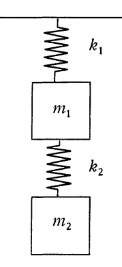
This post will look at simple numerical approaches to solving the predator-prey (Lotka-Volterra) equations. It turns out that the simplest approach does poorly, but a slight variation does much better.

Following [1] we will use the equations

u‘ = u (v − 2)
v‘ = v (1 − u)

Here u represents the predator population over time and v represents the prey population. When the prey v increase, the predators u increase, leading to a decrease in prey, which leads to a decrease in predators, etc. The exact solutions are periodic.

Euler’s method replaces the derivatives with finite difference approximations to compute the solution in increments of time of size h. The explicit Euler method applied to our example gives

u(t + h) = u(t) + h u(t) (v(t) − 2)
v(t + h) = v(t) + h v(t) (1 − u(t)).

The implicit Euler method gives

u(t + h) = u(t) + h u(t + h) (v(t + h) − 2)
v(t + h) = v(t) + h v(t + h) (1 − u(t + h)).

This method is implicit because the unknowns, the value of the solution at the next time step, appear on both sides of the equation. This means we’d either need to do some hand calculations first, if possible, to solve for the solutions at time t + h, or use a root-finding method at each time step to solve for the solutions.

Implicit methods are more difficult to implement, but they can have better numerical properties. See this post on stiff equations for an example where implicit Euler is much more stable than explicit Euler. I won’t plot the implicit Euler solutions here, but the implicit Euler method doesn’t do much better than the explicit Euler method in this example.

It turns out that a better approach than either explicit Euler or implicit Euler in our example is a compromise between the two: use explicit Euler to advance one component and use implicit Euler on the other. This is known as symplectic Euler for reasons I won’t get into here but would like to discuss in a future post.

If we use explicit Euler on the predator equation but implicit Euler on the prey equation we have

u(t + h) = u(t) + h u(t) (v(t + h) − 2)
v(t + h) = v(t) + h v(t + h) (1 − u(t)).

Conversely, if we use implicit Euler on the predator equation but explicit Euler on the prey equation we have

u(t + h) = u(t) + h u(t + h) (v(t) − 2)
v(t + h) = v(t) + h v(t) (1 − u(t + h)).

Let’s see how explicit Euler compares to either of the symplectic Euler methods.

First some initial setup.

    import numpy as np

    h  = 0.08  # Step size
    u0 = 6     # Initial condition
    v0 = 2     # Initial condition
    N  = 100   # Numer of time steps

    u = np.empty(N)
    v = np.empty(N)
    u[0] = u0
    v[0] = v0

Now the explicit Euler solution can be computed as follows.

    for n in range(N-1):
        u[n+1] = u[n] + h*u[n]*(v[n] - 2)
        v[n+1] = v[n] + h*v[n]*(1 - u[n])

The two symplectic Euler solutions are

    
    for n in range(N-1):
        v[n+1] = v[n]/(1 + h*(u[n] - 1))
        u[n+1] = u[n] + h*u[n]*(v[n+1] - 2)

and

    for n in range(N-1):
        u[n+1] = u[n] / (1 - h*(v[n] - 2))
        v[n+1] = v[n] + h*v[n]*(1 - u[n+1])

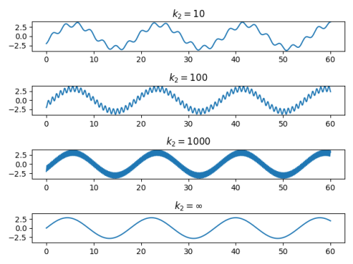
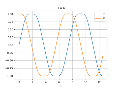
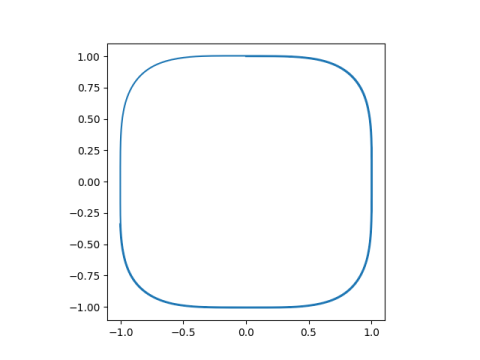
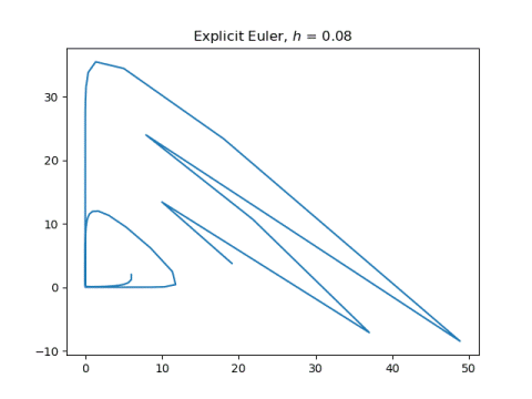
Now let’s see what our solutions look like, plotting (u(t), v(t)). First explicit Euler applied to both components:

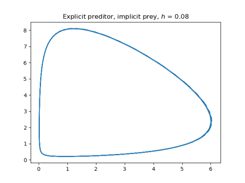
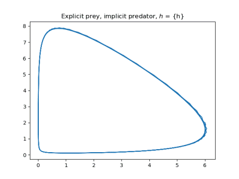
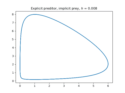
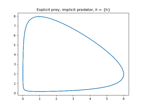
And now the two symplectic methods, applying explicit Euler to one component and implicit Euler to the other.

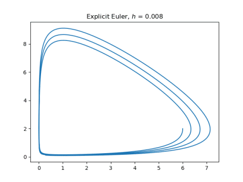
Next, let’s make the step size 10x smaller and the number of steps 10x larger.

Now the explicit Euler method does much better, though the solutions are still not quite periodic.

The symplectic method solutions hardly change. They just become a little smoother.

Leapfrog integrator

Posted on 13 July 2020 by John

The so-called “leapfrog” integrator is a numerical method for solving differential equations of the form

where x is a function of t. Typically x is position and t is time.

This form of equation is common for differential equations coming from mechanical systems. The form is more general than it may seem at first. It does not allow terms involving first-order derivatives, but these terms can often be eliminated via a change of variables. See this post for a way to eliminate first order terms from a linear ODE.

The leapfrog integrator is also known as the Störmer-Verlet method, or the Newton-Störmer-Verlet method, or the Newton-Störmer-Verlet-leapfrog method, or …

The leapfrog integrator has some advantages over, say, Runge-Kutta methods, because it is specialized for a particular (but important) class of equations. For one thing, it solves the second order ODE directly. Typically ODE solvers work on (systems of) first order equations: to solve a second order equation you turn it into a system of first order equations by introducing the first derivative of the solution as a new variable.

For another thing, it is reversible: if you advance the solution of an ODE from its initial condition to some future point, make that point your new initial condition, and reverse time, you can step back to exactly where you started, aside from any loss of accuracy due to floating point; in exact arithmetic, you’d return to exactly where you started.

Another advantage of the leapfrog integrator is that it approximately conserves energy. The leapfrog integrator could perform better over time compared to a method that is initially more accurate.

Here is the leapfrog method in a nutshell with step size h.

$\begin{align*} x_{i+1} &= x_i + v_i h + \frac{1}{2} f(x_i) h^2 \\ v_{i+i} &= v_i + \frac{1}{2}\left(f(x_i) + f(x_{i+1})\right) h \end{align*}$

And here’s a simple Python demo.

    import numpy as np
    import matplotlib.pyplot as plt
    
    # Solve x" = f(x) using leapfrog integrator
    
    # For this demo, x'' + x = 0
    # Exact solution is x(t) = sin(t)
    def f(x):
        return -x
    
    k = 5               # number of periods
    N = 16              # number of time steps per period
    h = 2*np.pi/N       # step size
    
    x = np.empty(k*N+1) # positions
    v = np.empty(k*N+1) # velocities
    
    # Initial conditions
    x[0] = 0
    v[0] = 1
    anew = f(x[0])
    
    # leapfrog method
    for i in range(1, k*N+1):
        aold = anew
        x[i] = x[i-1] + v[i-1]*h + 0.5*aold*h**2
        anew = f(x[i])
        v[i] = v[i-1] + 0.5*(aold + anew)*h

Here’s a plot of the solution over five periods.

There’s a lot more I hope to say about the leapfrog integrator and related methods in future posts.

Counterexample to Dirichlet principle

Posted on 11 July 2020 by John

Let Ω be an open set in some Euclidean space and v a real-valued function on Ω.

Dirichlet principle

Dirichlet’s integral for v, also called the Dirichlet energy of v, is

$\int_\Omega \frac{1}{2} | \nabla v |^2$

Among functions with specified values on the boundary of Ω, Dirichlet’s principle says that minimizing Dirichlet’s integral is equivalent to solving Laplace’s equation.

In a little more detail, let g be a continuous function on the boundary ∂Ω of the region Ω. A function u has minimum Dirichlet energy, subject to the requirement that u = g on ∂Ω, if and only if u solves Laplace’s equation

$\Delta; u = 0$

subject to the same boundary condition.

Dirichlet’s principle requires some hypotheses not stated here, as Hadamard’s example below shows.

Hadamard’s example

Let g(θ) be the function [1]

$g(\theta) = \sum_{n=1}^\infty \frac{\sin n!\theta}{n^2}$

The function g is continuous and so there exists a unique solution to Laplace’s equation on the unit disk with boundary values given by g, but the Dirichlet energy of the solution diverges.

The solution, in polar coordinates, is

$u(r, \theta) = \sum_{n=1}^\infty r^{n!} \,\,\frac{\sin n!\theta}{n^2}$

The Laplace operator in polar coordinates is

$\frac{1}{r} \frac{\partial }{\partial r}\left(r \frac{\partial u}{\partial r} \right) + \frac{1}{r^2} \frac{\partial^2 u}{\partial \theta^2}$

and you can differentiate u term by-term to show that it satisfies Laplace’s equation.

Dirichlet’s integral in polar coordinates is

$\int_0^{2\pi} \int_0^1 \frac{1}{2} \left\{ \left( \frac{\partial u}{\partial r}\right)^2 + \frac{1}{r^2}\left(\frac{\partial u}{\partial \theta}\right)^2 \right\} \, r\,dr\,d\theta$

Integrating term-by-term, the nth term in the series for the Dirichlet energy in Hadamard’s example is

$\frac{(n!)^2}{2n^4(2n! - 1)}$

and so the series rapidly diverges.

Dirichlet’s principle requires that there be at least one function satisfying the specified boundary conditions that has finite Dirichlet energy. In the example above, the solution to Laplace’s equation with boundary condition g has infinite Dirichlet energy. It turns out the same is true for every function satisfying the same boundary condition, whether it satisfies Laplace’s equation or not.

[1] What is the motivation for this function? The function is given by a lacunary series, a Fourier series with increasingly large gaps between the frequency components. The corresponding series for u cannot be extended to an analytic function outside the closed unit circle. If it could be so extended, Dirichlet’s principle would apply and the example wouldn’t work.

NASA’s favorite ODE solver

Posted on 16 June 2020 by John

NASA’s Orbital Flight Handbook, published in 1963, is a treasure trove of technical information, including a section comparing the strengths and weaknesses of several numerical methods for solving differential equations.

The winner was a predictor-corrector scheme known as Gauss-Jackson, a method I have not heard of outside of orbital mechanics, but one apparently particularly well suited to NASA’s needs.

The Gauss-Jackson second-sum method is strongly recommended for use in either Encke or Cowell [approaches to orbit modeling]. For comparable accuracy, it will allow step-sizes larger by factors of four or more than any of the forth order methods. … As compared with unsummed methods of comparable accuracy, the Gauss-Jackson method has the very important advantage that roundoff error growth is inhibited. … The Gauss-Jackson method is particularly suitable on orbits where infrequent changes in the step-size are necessary.

Here is a table summarizing the characteristics of each of the solvers.

Notice that Gauss-Jackson is the only method whose roundoff error accumulation is described as “excellent.”

A paper from 2004 [1] implies that the Gauss-Jackson method was still in use at NASA at the time of writing.

The Gauss-Jackson multi-step predictor-corrector method is widely used in numerical integration problems for astrodynamics and dynamical astronomy. The U.S. space surveillance centers have used an eighth-order Gauss-Jackson algorithm since the 1960s.

I could imagine a young hotshot explaining to NASA why they should use some other ODE solver, only to be told that the agency had already evaluated the alternatives half a century ago, and that the competitors didn’t have the same long-term accuracy.

Differential equations

Fourier, Gauss, and Heisenberg

Gaussian density

Heisenberg uncertainty

Related posts

A stiffening spring

Analytical solution

More differential equation posts

A generalization of sine and cosine

Odd order

Other generalizations of sine and cosine

Ripples and hyperbolas

More differential equation posts

Driving vibrations with sawtooth waves

Driving oscillations with square waves

Background

Exploration

Related posts

Symplectic Euler

More differential equations posts

Leapfrog integrator

More on ODE solvers

Counterexample to Dirichlet principle

Dirichlet principle

Hadamard’s example

Related posts

NASA’s favorite ODE solver

More math and space posts