Relations between special functions

The diagram below illustrates the relationships between many common special functions.

This page is a work in progress. Please contact me with corrections or suggestions.

The hypergeometric functon ₂F₁ has many special cases. (See these notes on hypergeometric functions for definitions and notation.)

The Jacobi polynomials are related to ₂F₁ by

$P^{(\alpha, \beta)}_n(z) = \frac{(a+1)^{\overline{n}}}{n!} F\left(-n, n+a+b+1; a+1; \frac{1-z}{2}\right)$

Jacobi polynomials with α = β are called Gegenbauer or ultraspherical polynomials and are denoted C^(α)_n. The Legendre polynomials P_n are Gegenbauer polynomials with α = 0. The Chebyshev polynomials of the first kind T_n are Gegenbauer polynomials with α = -½. The Chebyshev polynomials of the second kind U_n are Gegenbauer polynomials with α = ½.

The incomplete beta function B_x(a, b) is related to ₂F₁(x) by

$B_z(a,b) = z^a (1-z)^a\, F(1, a+b; a+1; z)$

The beta function B(a,b) is defined to be Γ(a) Γ(b) / Γ(a+b) and equals B₁(a, b).

The complete elliptic integrals K(z) and E(z) are related to ₂F₁ by

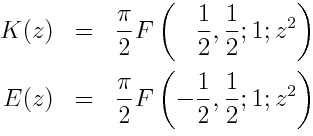
$K(z)=\frac{\pi}{2} F\left(\frac{1}{2}, \frac{1}{2}; 1; z^2\right) \\ E(z) = \frac{\pi}{2} F\left( -\frac{1}{2}, \frac{1}{2}; 1; z^2\right)$

The complete elliptic integrals are the values of the incomplete elliptic integrals F(φ, z) and E(φ, z) at φ = φ/2.

The inverse of the integral F(φ, z) is the Jacobi elliptic function sn. The Jacobi functions sn, cn, and dn are intimately related, much like the elementary trigonometric functions.

The hypergeometric functon ₁F₁ is also known as the confluent hypergeometric function. It is related to the hypergeometric function ₂F₁ by

$_1 F_1(a; c; z) = \lim_{b\to\infty} _2F_1(a, b; c; z/b)$

The incomplete gamma function γ(a, z) is related to ₁F₁ by

$\gamma(a, z) = \frac{z^a}{a} F(a; a+1; -z)$

The limit of γ(a, z) as z goes to infinity is the gamma function Γ(a).

The derivative of the logarithm of the gamma function Γ(z) is the function ψ(z).

The error function erf(z) is related to ₁F₁ by

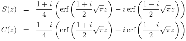
$\mbox{erf}(z) = z F\left(\frac{1}{2}; \frac{3}{2}; -z^2 \right)$

The error function erf(z) is related to the Fresnel integrals C(z) and S(z) by

The Laguerre polynomials L^α_n are related to ₁F₁ by

$L^\alpha_n(z) = \frac{(1+\alpha)^{\overline{n}}}{n!} F\left(-n; 1+\alpha}; z \right)$

The Hermite polynomials are related to the Laguerre polynomials by

$H_{2m}(z)=(-1)^m 2^{2m} m! L_m^{(-1/2)}(z^2) \\ H_{2m+1}(z) = (-1)^m 2^{2m+1} m! z L_m^{(1/2)}(z^2)$

The hypergeometric functon ₀F₁ is related to the hypergeometric function ₁F₁ by

$\lim_{a\to\infty} F\left(a; b; \frac{z}{a}\right) = \frac{2^{1-b}}{\Gamma(b)} F(\cdot ; b; z)$

Only Bessel functions of the first kind J_ν are shown on the diagram. Other Bessel functions are related to J_ν as described here.

Other diagrams on this site

See this page for more diagrams on this site including diagrams for probability and statistics, analysis, topology, and category theory.

Home