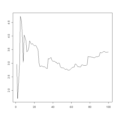
Suppose a Martian gives you a black box. It has a button on top and a display on the side. Every time you press the button, the box displays a number. You want to figure out the pattern to the numbers, so you make a record of the outputs and keep a running average. You hit the button 100 times, but the average keeps moving around. (There will be some theory further down the page, but first we start with some graphs to motivate the discussion.)

(The graph plots the cumulative sample average as a function of sample number.)
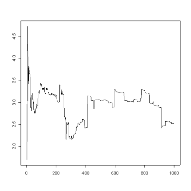
So you decide to keep going until you’ve hit the button 1000 times. Hmm, maybe the average is trending down lower than it looked like after 100 samples.

If we’d stopped after 4,000 samples we would have had a different idea of what’s going on than it looks after 10,000 samples. How do we know when to stop?
What kind of devilish box has the Martian given you? The samples used to create the graphs above were generated from a Cauchy(3, 1) distribution. The Cauchy distribution has the remarkable property that the average of N samples, for any positive integer N, has the same distribution as the original distribution. The average will not settle down no matter how many samples you take. That’s why the plots above have a fractal-like quality. The graphs will look similar no matter how many samples we take.
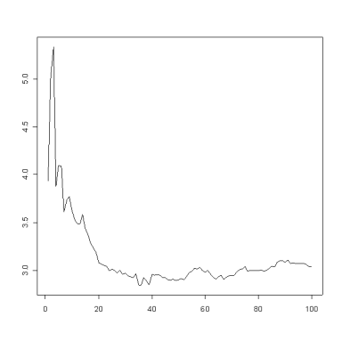
For a comparison, we will look briefly at the analogous graphs for a normal distribution. Here is a plot of the averages after each of the first 100 samples.

Unlike the Cauchy samples, the running average of the normal samples quickly converges to a nearly constant value.
The reason the sample mean for the Cauchy distribution is so erratic is that the Cauchy distribution has no mean for the sample mean to converge to. For any distribution that has a mean and a variance, the variance of the sample mean is inversely proportional to the number of samples. That’s why the running average for the normal settles down while the running average for the Cauchy keeps wandering.
For normal distributions, the sample mean converges to the population mean. The first time you see that result you may think “Well of course it does.” The example above helps show that there is substance to the normal sampling theory. The sample mean exists for the Cauchy even though the Cauchy itself does not have a mean.
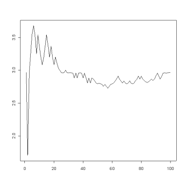
We would do better if we kept track of the median of our samples rather than the mean. Here are some plots of the sample median for the same Cauchy samples. After 100 samples we have the following.

The Cauchy distribution does have a median, and the sample median converges to that median. (Incidentally, the sample median would have worked well for normal samples, just not quite as well as the sample mean did.)
The distribution for the sample median of a Cauchy distribution is know. See Order Statistics, page 50. The book credits P. R. Rider, JASA 55: 322-3.
The PDF of the median of n = 2k + 1 samples from a standard Cauchy distribution is given below.
![]()
The variance of this distribution, given below, is finite for k ≥ 2.
![]()
