How should we define √(z² − 1)? Well, you could square z, subtract 1, and take the square root. What else would you do?!
The question turns out to be more subtle than it looks.
When x is a non-negative real number, √x is defined to be the non-negative real number whose square is x. When x is a complex number √x is defined to be a function that extends √x from the real line to the complex plane by analytic continuation. But we can’t extend √x as an analytic function to the entire complex plane ℂ. We have to choose to make a “cut” somewhere, and the conventional choice is to make a cut along the negative real axis.
Using the principal branch
The “principal branch” of the square root function is defined to be the unique function that analytically extends √x from the positive reals to ℂ \ (−∞, 0].
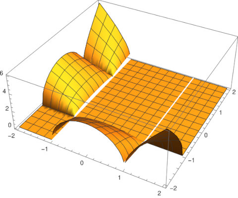
Assume for now that by √x we mean the principal branch of the square root function. Now what does √(z² − 1) mean? It could mean just what we said at the top of the post: we square z, subtract 1, and apply the (principal branch of the) square root function. If we do that, we must exclude those values of z such that (z² − 1) is negative. This means we have to cut out the imaginary axis and the interval [−1, 1].
This is what Mathematica will do when asked to evaluate Sqrt[z^2 - 1]. The command
ComplexPlot[Sqrt[z^2 - 1], {z, -2 - 2 I, 2 + 2 I}]
makes the branch cuts clear by abrupt changes in color.
A different approach
Now let’s take a different approach. Consider the function √(z² − 1) as a whole. Do not think of it procedurally as above, first squaring z etc. Instead, think of a it as a black box that takes in z and returns a complex number whose square is z² − 1.
This function has an obvious definition for z > 1. And we can extend this function, via analytic continuation, to more of the complex plane. We can do this directly, not by extending the square root function. But as before, we cannot extend the function analytically to all of ℂ. We have to cut something out. A common choice is to cut out [−1, 1]. This eliminates the need for a branch cut along the imaginary axis.
The function

extends √(z² − 1) the way we want [1].
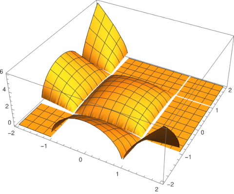
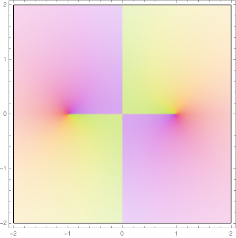
The Mathematica code
ComplexPlot[Exp[(1/2) (Log[z - 1 ] + Log[z + 1])], {z, -2 - 2 I, 2 + 2 I}]
shows that our function is now continuous across the imaginary axis, though there’s still a discontinuity as you cross [−1, 1].

We used this analytic extension of √(z² − 1) in the previous post to eliminate branch cuts in an identity.
Related posts
[1] The principal branch of the logarithm has a cut along the negative real axis. Why does our square root function, defined using log, not have a branch cut along the negative axis?
First of all, the log function, and Mathematica’s implementation of it Log[], isn’t undefined on (−∞, 1), it just isn’t continuous there. The function still has a value. By convention, the value is taken to be the limit of log(z) approaching z from above, i.e. from the 2nd quadrant.
Second, the value of (log(z – 1) + log(z + 1))/2 differs by a factor of 2πi when approaching a value z < −1 from above versus from below. This factor goes away when taking the exponential. So our function f(z) is analytic across (−∞, 1) even though the log functions in its definition are not.
![\left[ \begin{array}{cc|cc|cc|c} 0 & -1 & 0 & 0 & 0 & 0 & \cdots \\ 1 & 0 & 0 & 0 & 0 & 0 & \cdots \\ \hline 0 & 0 & 0 & -1 & 0 & 0 & \cdots \\ 0 & 0 & 1 & 0 & 0 & 0 & \cdots \\ \hline 0 & 0 & 0 & 0 & 0 & -1 & \cdots \\ 0 & 0 & 0 & 0 & 1 & 0 & \cdots \\ \hline \vdots & \vdots & \vdots & \vdots & \vdots & \vdots & \ddots \end{array} \right] \left[ \begin{array}{c} a_1 \\ b_1 \\ \hline a_2 \\ b_2 \\ \hline a_3 \\ b_3 \\ \hline \vdots \end{array} \right]](https://www.johndcook.com/hilbert_transform_matrix.svg)