Carl Jacobi’s advice to mathematicians was “always invert.” See what you can find out by turning a problem around. This post came from following Jacobi’s advice.
A few days ago I wrote a note about how you can approximate a normal probability density by one period of a cosine. Specifically, the approximation has density
f(x) = (1 + cos(x))/2 π.
for x between -π and π and zero outside that interval. This distribution has variance σ2 = π2/3 − 2 and so σ f(σx) is approximately a standard normal density.
Why approximate a normal density by a cosine? The cosine is more familiar than the normal density and can easily be integrated in closed form. The rule to always invert suggests it might be useful to approximate a cosine by a normal density.
What is a nice property of the normal density? For one thing, it is its own Fourier transform. So it might be worthwhile to approximate cosine by a normal density to have an idea what its Fourier transform looks like. Maybe the function σ f(σx) above doesn’t change too much when taking Fourier transforms. Is that right? Let’s look at a graph.
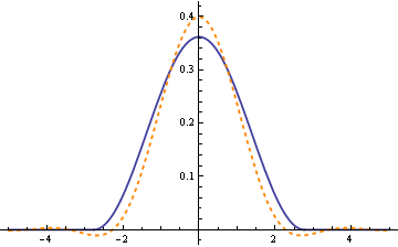
The solid blue line is σ f(σx) and the dashed orange line is its Fourier transform.
Other ideas
The cosine approximation for the normal density is more interesting than practical if your goal is simply to compute normal probabilities; there are more accurate approximations. But there are other uses of the cosine approximation, such as the example above. How else might you exploit the approximate relationship between sine waves and the normal distribution? I have the sense that there’s some application out there where this approximation swoops in and greatly simplifies a problem.
Update (6 May 2010): Here’s the Mathematica code used to create the graph above in PDF form. The code goes into more detail than the text of this post.
“What is a nice property of the normal density? For one thing, it is its own Fourier transform. So it might be worthwhile to approximate cosine by a normal density to have an idea what its Fourier transform looks like. ”
This is not going to work, because the Fourier transform of the normal density is a normal density only if you’re transforming from the whole real line to a whole real line. However, normal density is an approximation of the cosine on one period only. It is well-known what the Fourier transform of a cosine looks like — two Dirac delta functions — so the result of your approximation is completely wrong.
The idea of approximating a cosine by the normal density may have some uses, though.
Roman: You are right about the Fourier transform of cosine. I wasn’t clear about exactly what I was taking the transform of. I’m taking the Fourier transform over the whole real line of a function that is supported only on a finite interval. I updated the post to show the Mathematica code I was using. Thanks for prompting me to clarify this.
If cos approximates the normal distribution, then you might try approximating the normal cumulative function with the sine, and then finally the inverse cumulative with the arc sin. Would that be useful?
ST: Yes, that’s how you would use the approximation in a probability calculation.
At risk of firing off a half-baked idea – could this be applied to problems set in polar coordinates? If it can approximate the Normal, it should be able to approximate the von Mises distribution too.
…
Just had one of those “huh” moments where I notice a some of similarity between this approximation and the von Mises. Thanks John! :-)
Dear John,
If I understood you right the final approximation reads as follows (in Maple notation):
f(x) = (1/sigma)*(1/2)*(1+cos((1/sigma)*(x-mu)))/Pi
I am certainly going to read your reference of the 1961 paper “A cosine approximation to the normal distribution” by D. H. Raab and E. H. Green, Psychometrika, Volume 26, pages 447-450.
However, my question is as follows. How would the approximation look like for the bivariate case. For the bivariate standard normal distribution with standard normally distributed random variables X and Y one has E(XY) = r, where r is de correlation between X and Y. Would it be possible to construct a cosine bivariate approximation with the same property?