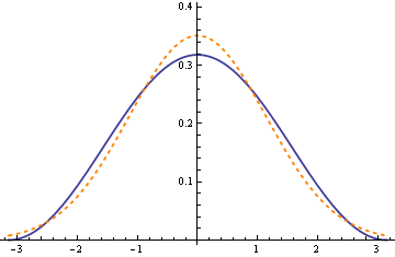
Here’s a simple approximation to the normal distribution I just ran across. The density function is
f(x) = (1 + cos(x))/2π
over the interval (−π, π). The plot below graphs this density with a solid blue line. For comparison, the density of a normal distribution with the same variance is plotted with a dashed orange line.
The approximation is good enough to use for teaching. Students may benefit from doing an exercise twice, once with this approximation and then again with the normal distribution. Having an approximation they can integrate in closed form may help take some of the mystery out of the normal distribution.
The approximation may have practical uses. The agreement between the PDFs isn’t great. However, the agreement between the CDFs (which is more important) is surprisingly good. The maximum difference between the two CDFs is only 0.018. (The differences between the PDFs oscillate, and so their integrals, the CDFs, are closer together.)
I ran across this approximation here. It goes back to the 1961 paper “A cosine approximation to the normal distribution” by D. H. Raab and E. H. Green, Psychometrika, Volume 26, pages 447-450.
Update 1: See the paper referenced in the first comment. It gives a much more accurate approximation using a logistic function. The cosine approximation is a little simpler and may be better for teaching. However, the logistic approximation has infinite support. That could be an advantage since students might be distracted by the finite support of the cosine approximation.
The logistic approximation for the standard normal CDF is
F(x) = 1/(1 + exp(−0.07056 x3 − 1.5976 x))
and has a maximum error of 0.00014 at x = ± 3.16.
Update 2: How might you use this approximation the other way around, approximating a cosine by a normal density? See Always invert.
Another interesting paper in this context:
http://www.jiem.org/index.php/jiem/article/download/60/27
There’s a history of these … There’s a famous approximation by Polya which I first learned of in the Chmura Kraemer and Thiemann book How Many Subjects?:
and an improvement in, I believe, a Master’s thesis by one Aludaat-Alodat:
Shucks… I tried to post images of these in the above. I know the first is correct. I believe the second, but I’m doing from memory. To see these, check out the links
http://bilge.pyrate.mailbolt.com/blogBeginningFriendship7Day2010/PolyaGaussian.png
and
http://bilge.pyrate.mailbolt.com/blogBeginningFriendship7Day2010/AludaatAlodatGaussian.png
Another nice approximation is the piecewise-cubic
M4 = M1 convolve M1 convolve M1 convolve M1
where M1(x) is the step function: 1 for x in -.5 .. .5, else 0.
Explicitly,
def M4(x):

    return (

          np.fmax( x+2, 0 ) ** 3

    - 4 * np.fmax( x+1, 0 ) ** 3

    + 6 * np.fmax( x, 0 ) ** 3

    - 4 * np.fmax( x-1, 0 ) ** 3

    +     np.fmax( x-2, 0 ) ** 3

    ) / 6
This comes from a lovely paper by I.J.Schoenberg, “On equidistant cubic spline interpolation”, Bulletin AMS, 1971.
cheers
— denis
Folklore has it that an early IBM standard normal distribution pseudo-random number generator was the sum of twelve [0,1] uniform pseudo-random numbers minus 6. A straight-forward application of the central limit theorem.
For more on generating a normal random variable from twelve uniform variables, see this post and the comments.
Which approximation gives us moments that are close approximations to the real moments?
The normal distribution is only important in statistical inference, so the core is irrelevant and the tails are of the utmost importance. The normal is both skewed and kurtotic until the sample is large enough to achieve normality. Until that normality is reached, one tail is long and the other tail is short. The cosine is only mythically approximate and only so after the sample is large.
If you were putting money on it, put it on the short tail side of the distribution, because the probability mass is moving in that direction. The cosine approximation will leave you clueless.
Re: James @ 11:45
It’s not folklore. I clearly remember that the IBM 1130 FORTRAN library used the sum of 12 uniform[0, 1] pseudorandom variates to generate a Gaussian PR variate. We ran into a problem because of this. We were simulating communication systems in which errors were caused by additive white gaussian noise. Well, if one uses the IBM library gaussian function, the results are badly wrong at high signal to noise ratio.
The absolute error is small but the relative error starts growing at about 2.5 standard deviations.
Luckily for us, the errors were so great that it was obvious that something was wrong.