This afternoon I got a review copy of the book Creating Symmetry: The Artful Mathematics of Wallpaper Patterns. Here’s a striking curves from near the beginning of the book, one that the author calls the “mystery curve.”
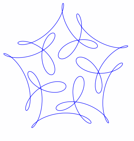
The curve is the plot of exp(it) − exp(6it)/2 + i exp(−14it)/3 with t running from 0 to 2π.
Here’s Python code to draw the curve.
    import matplotlib.pyplot as plt
    from numpy import pi, exp, real, imag, linspace

    def f(t):
        return exp(1j*t) - exp(6j*t)/2 + 1j*exp(-14j*t)/3

    t = linspace(0, 2*pi, 1000)

    plt.plot(real(f(t)), imag(f(t)))

    # These two lines make the aspect ratio square
    fig = plt.gcf()
    fig.gca().set_aspect('equal')

    plt.show()
Maybe there’s a more direct way to plot curves in the complex plane rather than taking real and imaginary parts.
Updated code for the aspect ratio per Janne’s suggestion in the comments.
Similar posts
Several people have been making fun visualizations that generalize the example above.
Brent Yorgey has written two posts, one choosing frequencies randomly and another that animates the path of a particle along the curve and shows how the frequency components each contribute to the motion.
Mike Croucher developed a Jupyter notebook that lets you vary the frequency components with sliders.
John Golden created visualizations in GeoGerba here and here.
Dan Anderson accused me of nerd sniping him and created this visualization.
It looks like the kind of thing Spirograph would have produced, except that the loops are of varying sizes. I wonder whether Spirograph with the ring moving as you draw could produce something like this.
The axes(“equal”) convenience function will do what you want. Or, to fit your code nicely and do it more explicitly:
fig.gca().set_aspect('equal')If you do the second one in an interactive session you also have to trigger an update for the change to take effect.
It is a lovely looking curve. Its pentagonal symmetry is clearer if the function is
written as exp(it)*[ 1 – exp(i*5*t)/2 + i*exp(i*15*t)/3], so every 2*pi/5 we generate the same shape rotated by 2*pi/5. I’m not sure why it’s called a mystery curve, though.
Oops, I forgot to type the minus sign inside that last exponential.
Very nice, thanks.
But how did you know that’s the equation for that curve? I’m guessing it’s not quite as simple as fitting a polynomial :)
I was a little baffled when you said “Maybe there’s a more direct way to plot curves in the complex plane rather than taking real and imaginary parts.” How else would you plot something in the complex plane? Isn’t one axis real, and one imaginary? That’s the only version of the complex plane to which I’ve been exposed – is there another take on the complex plane of which I’m unaware?
Matthew: I meant maybe there’s a plotting command that could take the vector of complex values as input and and plot it directly, not requiring the user to explicitly plot real and imaginary parts. There is such a command in Sage. I believe it’s list_plot or something like that. But as far as I know there’s no such command in matplotlib.
Dr. Cook – Oh, ok. That makes sense. Thanks for clarifying.
Neat. There are many entertaining curves based on this just by changing the symmetry, e.g.:
import matplotlib.pyplot as plt

from numpy import pi, exp, real, imag, linspace
def P(u):
return 1 - u/2 + 1j*(u**-3)/3
def f(t,k):
return exp(1j*t)*P(exp(k*1j*t))
t = linspace(0,2*pi, 1001);
# Integer k
k = 12
plt.plot(real(f(t,k)), imag(f(t,k)))
plt.show()
k = -5 is also amusing.
Here’s the formula for Spirograph-type curves, created by rolling one disk inside or outside another.
import matplotlib.pyplot as plt
from numpy import pi, exp, real, imag, linspace

def spiro(t, r1, r2, r3):
    """
    Create Spirograph curves made by one circle of radius r2 rolling
    around the inside (or outside) of another of radius r1.  The pen
    is a distance r3 from the center of the first circle.
    """
    return r3*exp(1j*t*(r1+r2)/r2) + (r1+r2)*exp(1j*t)

def circle(t, r):
    return r * exp(1j*t)

r1 = 96.0
r2 = -52.0
r3 = 42.0
ncycle = 13 # LCM(r1,r2)/r2

t = linspace(0, ncycle*2*pi, 1000)
plt.plot(real(spiro(t, r1, r2, r3)), imag(spiro(t, r1, r2, r3)))
plt.plot(real(circle(t, r1)), imag(circle(t, r1)))

fig = plt.gcf()
fig.gca().set_aspect('equal')
plt.show()
With values of
… you can produce the default curve on Nathan Friend’s Inspirograph app.
Thanks for the post and book recommendation. I’ve been going down the Sacred Geometry rabbit hole using a bow compass and straightedge to create really interesting designs. It’s brought me to books like “Islamic Design – A Genius for Geometry” http://www.amazon.com/Islamic-Design-Genius-Geometry-Wooden/dp/0802716350/ref=sr_1_6?s=books&ie=UTF8&qid=1435240870&sr=1-6&keywords=islamic+patterns
I’ll be getting the book you suggested.
On another note, I’ve been tinkering with the PowerShell C# app that does logo. It’s interesting to do do these designs programmatically. By hand, I feel more like a participant though.
Thanks again.
Doug