Ten years ago I wrote about how cosine makes a decent approximation to the normal (Gaussian) probability density. It turns out you get a much better approximation if you raise cosine to a power.
If we normalize cosk(t) by dividing by its integral
![]()
we get an approximation to the density function for a normal distribution with mean 0 and variance 1/k.
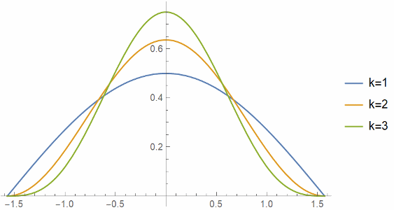
Here are the plots of cosk(t), normalized to integrate to 1, for k = 1, 2, and 3.
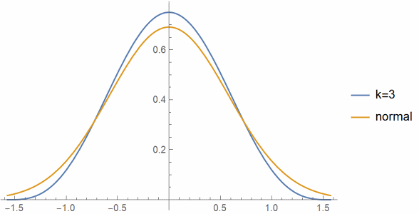
And here’s a plot of cos3(t) compared to a normal with variance 1/3.
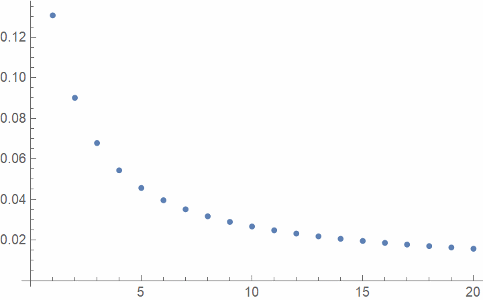
And finally here’s a plot of L² error, the square root of the integral of the square of the approximation error, as a function of k.
Update: You can do much better if you take a convex combination of cosine with 1 and allow non-integer powers. See this post.
This is somewhat interesting because normal distributions are all rescalings of one another, but powers of cosine clearly are not.
Which value of k gives the best approximation? The L^2 error seems to be strictly decreasing, but that reflects the effect of scaling; expanding the x axis by a factor of k, but shrinking the y axis by the same factor, reduces the L^2 norm of a function by sqrt(k), so it would be more natural to plot the L^2 error times sqrt(k) if you want to compare apples to apples.
If you normalize the cosine power so that it has unit variance, i.e. take cos(x/sqrt(p))^p, one can show that in the limit p->inf one recovers the normal probability density (up to the 1/sqrt(2pi) constant).