The last couple posts have been looking at the logistic bifurcation diagram a little at a time.
The first post in the series looked at the details of that part of the diagram that looks like the graph of a function, where there parameter r in the logistic map
f(x) = r x(1 − x)
varies from o to 3.
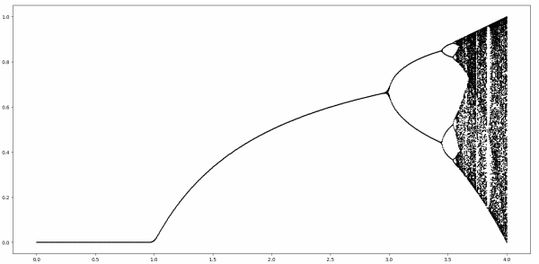
The first branch point occurs at r = 3. When r is exactly equal to 3, almost all starting points converge to the same point, though they converge very slowly. When r is slightly larger than 3 the (stable) iterates no longer converge to a point but instead oscillate between two points.
The second post in this series looked at the first fork, corresponding to values of r from 3 to 1 + √6. For r larger than 1 + √6 the previous stable cycle points become unstable and split into two new cycles each. These new cycles will split (“bifurcate”) into two new cycles, and so on and so on until there are infinitely many cycles and chaos breaks out around r = 3.56995.
This post will look at the horizontal spacing between branch points.
The first branch point occurs when r equals b1 = 3.
The two branches branch again when r crosses b2 = 1 + √6.
The next branch point is b3 = 3.5440903…. Why is there a simple expression for b1 and b2 but not for b3? Everything gets more complicated as r increases. The number b3 is algebraic, the root of a 12th degree polynomial [1].
t12 − 12t11 + 48t10 − 40t9 − 193t8 + 392t7 + 44t6 + 8t5 − 977t4 − 604t3 + 2108t2 + 4913 = 0
The number b4 has algebraic also been shown to be algebraic: someone found a 120-degree polynomial with integer coefficients such that −b4(b4 − 2) is a root [1]. The coefficients in the polynomial vary over 72 orders of magnitude. Perhaps its possible to find polynomials with other branch points as roots, but this doesn’t seem promising or practical.
The spacing between branch points decreases rapidly, becoming infinitely small before chaos breaks out. The ratio of spacings between consecutive branch points converges to a constant, known as Feigenbaum’s constant
δ = 4.66920…
This constant is known to surprising precision. Directly computing the constant to high precision by numerically finding branch points would be impractical, but Feigenbaum came up with an indirect way of computing his constant via a functional equation. The constant δ has been computed at least 1018 digits.
Feigenbaum’s constant does not just apply to the iterations of the logistic map. It’s a “universal” constant in that it applies to a class of dynamical systems.
Previous posts in this series
[1] Jonathan Borwein and David Bailey. Mathematics by Experiment: Plausible Reasoning in the 21st Century. 2004.