Inverting matrices and bilinear functions

The inverse of the matrix

$M = \begin{bmatrix} a & b \\ c & d \end{bmatrix}$

is the matrix

$M^{-1} = \frac{1}{|M|} \begin{bmatrix} d & -b \\ -c & a \end{bmatrix} = \frac{1}{ad - bc} \begin{bmatrix} d & -b \\ -c & a \end{bmatrix}$

assuming ad − bc ≠ 0.

Also, the inverse of the bilinear function (a.k.a. Möbius transformation)

$f(z) = \frac{az + b}{cz + d}$

is the function

$f^{-1}(z) = \frac{dz - b}{-cz + a}$

again assuming ad − bc ≠ 0.

The elementary takeaway is that here are two useful equations that are similar in appearance, so memorizing one makes it easy to memorize the other. We could stop there, but let’s dig a little deeper.

There is apparently an association between 2 × 2 matrices and Möbius transformations

$\frac{az + b}{cz + d} \leftrightarrow \begin{bmatrix} a & b \\ c & d \end{bmatrix}$

This association is so strong that we can use it to compute the inverse of a Möbius transformation by going to the associated matrix, inverting it, and going back to a Möbius transformation. In diagram form, we have the following

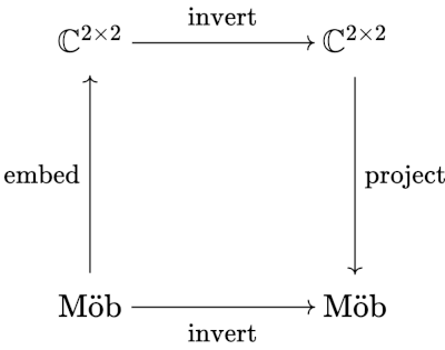
Now there are a few lose ends. First of all, we don’t really have a map between Möbius transformations and matrices per se; we have a map between a particular representation of a Möbius transformation and a 2 × 2 matrix. If we multiplied a, b, c, and d in a Möbius transformation by 10, for example, we’d still have the same transformation, just a different representation, but it would go to a different matrix.

What we really have a map between Möbius transformations and equivalence classes of invertible matrices, where two matrices are equivalent if one is a non-zero multiple of the other. If we wanted to make the diagram above more rigorous, we’d replace ℂ^2×2 with PL(2, ℂ), linear transformations on the complex projective plane. In sophisticated terms, our map between Möbius transformations and matrices is an isomorphism between automorphisms of the Riemann sphere and PL(2, ℂ).

Möbius transformations act a lot like linear transformations because they are linear transformations, but on the complex projective plane, not on the complex numbers. More on that here.

Leave a Reply