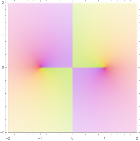
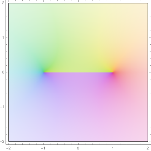
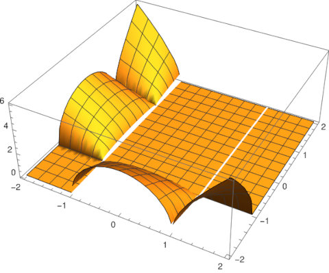
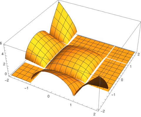
Airfoils

Here’s something surprising: You can apply a symmetric function to a symmetric shape and get something out that is not symmetric.

Let f(z) be the average of z and its reciprocal:

f(z) = (z + 1/z)/2.

This function is symmetric in that it sends z and 1/z to the same value.

Now apply f to circles in the complex plane, varying the center and the radius. Here are some examples of what the image of circles are.

These shapes look a lot like a cross section of an airplane wing, i.e.an airfoil. You can vary the radius of the circle to change the thickness of the airfoil and you can vary the imaginary part of the center to control the camber, how much the center of the airfoil bends [1].

The reason the symmetric function f applied to a symmetric shape can give a non-symmetric shape is that the word “symmetric” is being used in different senses. Still, it is surprising to see a complicated shape pop out of a simple function applied to a simple shape. Also, although the circle is perfectly smooth, the image of the circle has a sharp cusp. This is because the circles include or approach the singularity of f at 0.

The function f above is called the Joukowsky transformation, named after Nicolai Joukowsky (Никола́й Жуко́вский) who published its application to airfoils in 1910. The Joukowsky transformation gives a conformal map between a disk and an airfoil. This map lets engineers map problems from the difficult geometry of an airfoil to the simple geometry of a disk, and then map back to the airfoil. You could design an airfoil to have the shape of the transformation of a circle, or you could design a transformation so that the image of a circle approximates your airfoil.

The function f doesn’t map every circle to an airfoil-like shape, though of course aerospace engineers are most interested in the case where you do. Also, in the examples above the trailing edge of the airfoil comes to a cusp. This is not always the case; you can adjust the circle so that you have a more rounded trailing edge. The following plot illustrates both these possibilities.

More conformal mapping posts

[1] The thickness of the airfoil doesn’t depend on the radius R so much as the ratio R/a where the circle has center

c = aR exp(-iβ).

The ratio R/a is related to the thickness, and the parameter β is related to the camber.

Bounds on power series coefficients

Let f be an analytic function on the unit disk with f(0) = 0 and derivative f ′(0) = 1. If f is one-to-one (injective) then this puts a strict limit on the size of the series coefficients.

Let an be the nth coefficient in the power series for f centered at 0. If f is one-to-one then |an| ≤ n for all positive n. Or to put it another way, if |an| > n for any n > 0 then f must take on some value twice.

The statement above was originally known as the Bieberbach conjecture, but is now known as De Branges’ theorem. Ludwig Bieberbach came up with the conjecture in 1916 and Louis de Branges proved it in 1984. Many people between Bieberbach and De Branges made progress toward the final theorem: proving the theorem for some coefficients, proving it under additional hypotheses, proving approximate versions of the theorem, etc.

The function f(z) = z /(1 – z)² shows that the upper bound in De Branges’ theorem is tight. This function is one-to-one on the unit interval, and its nth coefficient is equal to n.

Jacobi functions with complex parameter

Jacobi functions are complex-valued functions of a complex variable z and a parameter m. Often this parameter is real, and 0 ≤ m < 1. Mathematical software libraries, like Python’s SciPy, often have this restriction. However, m could be any complex number.

The previous couple of posts spoke of the fundamental rectangle for Jacobi functions. But in general, Jacobi functions (and all other elliptic functions) have a fundamental parallelogram.

When m is real, the two periods of the Jacobi sn function are 4K(m) and 2K(1-m) i and so the function repeats horizontally and vertically. (Here K is the complete elliptic integral of the first kind.) When m is complex, the two periods are again 4K(m) and 2K(1-m) i, but now 4K(m) and 2K(1-m) are complex numbers and their ratio is not necessarily real. This means sn repeats over a parallelogram which is not necessarily a rectangle.

The rest of the post will illustrate this with plots.

First, here is a plot of sn(K(1/2)z, 1/2). The height of the graph represents the absolute value of the function and the color represents its phase. (The argument z was multiplied by K(1/2) to make the periods have integer values, making it a little easier to see the periods.)

Notice that the plot features line up with the coordinate axes, the real axis running from 0 to 8 in the image and the complex axis running from 0 to 4.

Here’s the analogous plot for sn(z, 2 + 2i).

Now the features are running on a diagonal. The pits are where the function is zero and the white ellipses are poles that have have the tops cut off to fit in a finite plot.

It will be easier to see what’s going on if we switch to flat plots. The color represents phase as before, but now magnitude is denoted by contour lines.

Here’s a plot of sn(K(1/2)z, 1/2)

and here’s a plot of sn(z, 2 + 2i).

According to theory the two periods should be

4 K(2 + 2i) = 4.59117 + 2.89266 i

and

2i K(-1 – 2i) = -1.44633 + 2.29559 i.

We can show that this is the case by plotting the real and imaginary parts of sn(z, 2 + 2i) as we move in these two directions.

The Mathematica code

    Plot[
        {Re[JacobiSN[t EllipticK[2 + 2 I], (2 + 2 I)]],
         Im[JacobiSN[t EllipticK[2 + 2 I], (2 + 2 I)]]}, 
        {t, 0, 4}]

produces this plot

and the code

    Plot[
        {Re[JacobiSN[t I EllipticK[-1 - 2 I], (2 + 2 I)]], 
         Im[JacobiSN[t I EllipticK[-1 - 2 I], (2 + 2 I)]]}, 
        {t, 0, 4}]

produces this plot.

Related posts

Conformal map from rectangles to half plane

As discussed in the previous post, the Jacobi elliptic function sn(z, m) is doubly periodic in the complex plane, with period 4K(m) in the horizontal direction and period 2K(1-m) in the vertical direction. Here K is the complete elliptic integral of the first kind.

The function sn(z, m) maps the rectangle

(-K(m), K(m)) × (0, K(1-m))

conformally onto to the upper half plane, i.e. points in the complex plane with non-negative imaginary part.

For example, sn(z, 0.5) takes the rectangle

to

The function sn has a singularity at the top middle of the rectangle, and so as horizontal lines approach the top of the rectangle, their image turns into bigger and bigger circles. filling the half plane.

The plot above was created with the following Mathematica code:

    K = EllipticK[1/2]
    Show[
        ParametricPlot[
            Table[{Re[JacobiSN[x + I y, 0.5]], Im[JacobiSN[x + I y, 0.5]]}, 
            {x, -K, K, K/10}], {y, 0, K}], 
        ParametricPlot[
             Table[{Re[JacobiSN[x + I y, 0.5]], Im[JacobiSN[x + I y, 0.5]]}, 
             {y, 0, K, K/10}], {x, -K, K}], 
        PlotRange -> {{-8, 8}, {0, 8}}]

You can vary the parameter m to match the shape of the rectangle you want to map to the half plane. You cannot choose both the length and width of your rectangle with only one parameter, but you can choose the aspect ratio. By choosing m = 1/2 we got a rectangle twice as wide as it is tall.

In our example we have a rectangle 3.70815 wide and 1.85407 tall. If we wanted a different size but the same aspect ratio, we could scale the argument to sn. For example,

sn(Kz, 0.5)

would map the rectangle (-1, 1) × (0, 1) onto the open half plane where K is given in the Mathematica code above.

In general we can solve for the parameter m that gives us the desired aspect ratio, as explained in the previous post, then find k such that sn(kz, m) maps the rectangle of the size we want into the half plane.

The inverse function, mapping the half plane to the rectangle, can be found in terms of elliptic integrals. Mathematica provides a convenient function InverseJacobiSN for this.

We could map any rectangle conformally to any other rectangle by mapping the first rectangle to the upper half plane, then mapping the upper half plane to the second rectangle. (We can’t simply scale the rectangle directly because such a map will not be conformal, will not preserve angles, unless we scale horizontally and vertically by the same amount. We can find a conformal map that will change the aspect ratio of a rectangle, but it will not simply scale the rectangle linearly.)

Although we can conformally map between any two rectangles using the process described above, we may not want to do things this way; the result may not be what we expect. Conformal maps between regions are not quite unique. They are unique if you specify where one point in the domain goes and specify the argument of its derivative. You may need to play with those extra degrees of freedom to get a conformal map that behaves as you expect.

Related posts

Conformal map of rectangle to ellipse

The previous post looked at what the sine function does to circles in the complex plane. This post will look at what it does to an rectangle.

The sine function takes a rectangle of the form [0, 2π] × [0, q] to an ellipse with semi major axis cosh(q) and semi minor axis sinh(q).

The image of horizontal lines

is a set of concentric ellipses.

The sine function almost maps the interior of the rectangle to the interior of the ellipse.

If we add vertical lines to the rectangle

the results are a little puzzling.

The images of the dashed green vertical lines seem broken in the ellipse. Their images above the real axis don’t line up with their images below the real axis. This isn’t easy to see on the edges, but you can see it in the middle. There are 20 green lines in the preimage but 19 in the image. That’s because sine maps both vertical edges of the rectangle to the same line segment in the image.

It will be clearer if we make our rectangle slightly narrower, changing the base from [0, 2π] to [0, 6].

Now notice the split in the image;

Now we can see what’s going on. Sine doesn’t distort the rectangle into an ellipse from the inside out, not like the map between a circle and an ellipse. Instead it maps the left edge of the rectangle along the imaginary axis, then bends the rectangle around the real axis clockwise, then back around the real axis.

So sine conformally maps the interior of the rectangle, the open rectangle (0, 2π) × (0, q) to the interior of the ellipse with a couple slits removed, one slit along the positive imaginary axis and another slit along the real axis from -1 to 1.

So how would you map the interior of a rectangle to the interior of an ellipse with no slits? For the special case of a square, you could compose the maps from two previous posts: map the square to a disk, then map the disk to an ellipse.

Related posts

Sine of a circle

What does it look like when you take the sine of a circle? Not the angle of points on a circle, but the circle itself as a set of points in the complex plane?

Here’s a plot for the sine of circles of radius r centered at the origin, 0 < r < π/2.

Here’s the same plot but for π/2 < r < π.

Now let’s see what happens when we shift the center of the circle over by 1, first for 0 < r < π/2.

And now for π/2 < r < π.

Here’s the Python code that produced the first plot; the code for the other plots is very similar.

    import matplotlib.pyplot as plt
    from numpy import pi, exp, sin, linspace

    t = linspace(0, 2*pi, 500)

    for r in linspace(0.1, pi/2, 17):
        z = r*exp(1j*t) 
        w = sin(z)
        plt.plot(w.real, w.imag, 'b')

    plt.gca().set_aspect("equal")
    plt.title("$\sin(r\exp(it))$, $0 < r < \pi/2$")
    plt.show()

Related posts

Test whether three complex numbers are vertices of an equilateral triangle

Let a, b, and c be three complex numbers.

Triangle with vertices at exp(pi/12), exp(9pi/12), and exp(17pi/12).

These numbers form the vertices of an equilateral triangle in the complex plane if and only if

\left| \begin{matrix} a & b & 1 \\ b & c & 1 \\ c & a & 1 \\ \end{matrix} \right| = 0

This theorem can be found in [1].

If we rotate the matrix above, we multiply its sign by -1. If we then swap two rows we multiply the determinant again by -1. So we could write the criterion above with the 1’s on the top row.

\left| \begin{matrix} 1 & 1 & 1 \\ a & b & c \\ b & c & a \\ \end{matrix} \right| = 0

See also this post which gives the area of a triangle in the complex plane, also in terms of a determinant.

[1] Richard Deaux. Introduction to the Geometry of Complex Numbers.

Area of a triangle in the complex plane

I recently ran across an elegant equation for the area of a triangle in the complex plane with vertices at z1, z2, and z3. [1].

A(z_1, z_2, z_3) = \frac{i}{4} \, \left| \begin{matrix} z_1 & \bar{z}_1 & 1 \\ z_2 & \bar{z}_2 & 1 \\ z_3 & \bar{z}_3 & 1 \\ \end{matrix} \right|

This formula gives the signed area: the area is positive if the points are given in countclockwise order and negative otherwise.

I’ll illustrate the formula with a little Python code. Let’s generate a random triangle.

    import numpy as np

    np.random.seed(20221204)
    r = 100*np.random.random(6)
    z1 = r[0] + 1j*r[1]
    z2 = r[2] + 1j*r[3]
    z3 = r[4] + 1j*r[5]

Here’s what our triangle looks like plotted.

Now let’s calculate the area using the formula above and using Heron’s formula.

    
    def area_det(z1, z2, z3):
        det = 0
        det += z2*z3.conjugate() - z3*z2.conjugate()
        det -= z1*z3.conjugate() - z3*z1.conjugate()
        det += z1*z2.conjugate() - z2*z1.conjugate()
        return 0.25j*det
    
    def area_heron(z1, z2, z3):
        a = abs(z1-z2)
        b = abs(z2-z3)
        c = abs(z3-z1)
        s = 0.5*(a + b + c)
        return np.sqrt(s*(s-a)*(s-b)*(s-c))
        
    print(area_heron(z1, z2, z3))
    print(area_det(z1, z2, z3))

This prints -209.728 and 209.728. The determinate gives a negative area because it was given the points in clockwise order.

[1] Philip J. Davis. Triangle Formulas in the Complex Plane. Mathematics of Computation. January 1964.

Conformal map between square and disk

Conformal maps transform one region into another while preserving angles. You might solve a PDE, for example, by mapping it to a standard region, solving it there, then mapping the solution back to the original region.

Some tasks are easier to do in a square and others in a disk, so it’s clearly useful to be able to conformally map between squares and disks. The Riemann mapping theorem tells us this can be done, but it doesn’t tell us how. Two gentlemen figured out how to map between squares (and more general polygons) and disks in the 1860s: Hermann Schwarz and Elwin Christoffel. Schwarz is known for many different results in analysis, including the topic of the previous post, the conformal map from an ellipse to the unit disk. Christoffel is best known for Christoffel symbols, building blocks of tensors.

Here’s a plot showing how the Schwarz-Christoffel transformation from the square [-1, 1] × [-1, 1] to the unit disk transforms Cartesian grid lines.

Here’s another plot, this one showing how the grid lines for polar coordinates on the disk pull back to curves on the square.

Equations

The equation for the function from the square to the disk is

f(z) = \frac{1-i}{2} \, \text{sd}\left(\frac{1+i}{2} K z;\frac{1}{2}\right)

where sd is a Jacobi elliptic function with parameter 1/2 [1]. The constant K is the complete elliptic function of the first kind, evaluated at 1/2. In symbols, K = K(1/2).

The inverse function has equation

g(w) = (1-i) - \frac{1-i}{K} F\left(\cos^{-1}\left(\frac{1-i}{\sqrt{2}} w\right);\frac{1}{2} \right )

Here F is the incomplete elliptic function of the first kind. For more background, see this post on kinds of elliptic integrals.

Fast approximation

An exact map from the square to the disk requires elliptic functions. However, there is a simple polynomial approximation to the map above [2].

f(z) \approx z + 0.0731647\,z + 0.00358709\,z^9

Peirce’s projection

Charles Sanders Peirce used the conformal map of the disk to the square to create the “Peirce quincuncial projection” map. This is a conformal (i.e. angle-preserving) map that represents the globe on a square. The diamond shape in the middle is the image of the equator. The mapping is singular at the south pole.

Charles Sanders Peirce's quincuncial project

Peirce named the map after the quincunx pattern of the poles. This obscure word refers to the pattern of dots on the five face of a standard six-sided die.

⚄

Related posts

[1] “Parameter” is being used in a technical sense here. There are two conventions for describing the parameterization of elliptic functions and elliptic functions and elliptic integrals, and here we are using the parameter called The Parameter, commonly denoted m. There’s another convention that uses the elliptic modulus k, and the connection between them is that m = k².

[2] Prem K. Kythe. Handbook of Conformal Mappings and Applications. CRC Press. Page 286.

Conformal map of ellipse interior to a disk

This post will present the conformal map between the interior of an ellipse and the unit disk.

Given an ellipse centered at the origin with semi-major axis a and semi-minor axis b. Will will assume without loss of generality that a² – b² = 1 and so the foci are at ±1.

Hermann Schwarz published the conformal map from the ellipse to the unit disk in 1869 [1, 2].

The map is given by

f(z) = \sqrt{k}\,\, \text{sn} \left( \frac{2K}{\pi} \sin^{-1}(z) \right)

where sn is the Jacobi elliptic function with parameter k². The constants k and K are given by

\begin{align*} q &= (a + b)^{-4} \\ k &= \left(\frac{\theta_2(q)}{\theta_3(q)}\right)^2 \\ K &= \frac{\pi}{2} \theta_3(q)^2 \end{align*}

where θ2 and θ3 are theta constants, the value so the theta functions θ2(z, q) and θ3(z, q) at z = 1.

Conformal maps to the unit disk are unique up to rotation. The map above is the unique conformal map preserving orientation:

\begin{align*} f(0) &= 0 \\ f(\pm a) &= \pm 1 \\ f(\pm bi) &= \pm i \\ \end{align*}

Inverse map

The inverse of this map is given by

g(w) = \sin\left(\frac{\pi}{2K} \,\, \text{sn}^{-1} \left(\frac{w}{\sqrt{k}}\right) \right)

The inverse of the sn function with parameter m can be written in terms of elliptic integrals.

\text{sn}^{-1}(z; m) = F\left(\sin^{-1}(u; m)\right)

where F is the incomplete elliptic integral of the first kind and m is the parameter of sn and the parameter of F.

Plot

I wanted to illustrate the conformal map using an ellipse with aspect ratio 1/2. To satisfy a² – b² = 1, I set a = 2/√3 and b = 1/√3. The plot at the top of the post was made using Mathematica.

Related posts

[1] H. A. Schwarz, Über eigige Abbildungsaufgaben, Journal für di reine und angew. Matheamatik, vol 70 (1869), pp 105–120

[2] Gabor Szegö. Conformal Mapping of the Interior of an Ellipse onto a Circle. The American Mathematical Monthly, 1950, Vol. 57, No. 7, pp. 474–478