Estimating a cumulative sum

In this post I mentioned two series which I denoted t(n) and c(n). The former is the number of unlabeled rooted trees with n nodes. The latter is the cumulative sum of the former, i.e.

$c(n) = t(1) + t(2) + t(3) + \cdots + t(n)$

The sequence c(n) is also the number of constrains on an n-step Runge-Kutta method; that’s how I became interested in it.

Now the t(n) sequence has been cataloged as OEIS A000081 and OEIS gives the asymptotic estimate of t(n) for large n as

$t(n) \sim C \frac{a^n}{n^{3/2}}$

where C = 0.4399… and α = 2.9557….

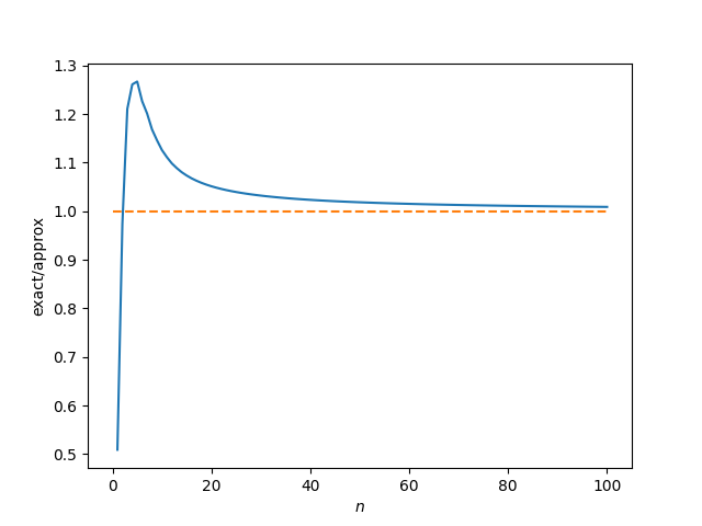
The cumulative sum of t(n), what I’ve called c(n), is also cataloged in OEIS, sequence number A087803. However, OEIS does not give an asymptotic estimate for this sequence. I’ll give one here.

(Update: After looking closer at the page for A087803 I see that there is an asymptotic formula, the same one derived here.)

The basis for my derivation is to assume the cumulative sum of the asymptotic estimates gives an asymptotic estimate of the cumulative sum. This is justified by the fact that the sequence is increasing rapidly and only the last few terms contribute much relatively to the sum.

The technique illustrated here would be applicable to the cumulative sum of other series whose asymptotic form is known.

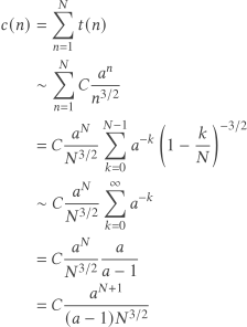
$\begin{align*} c(n) &= \sum_{n=1}^N t(n) \\ &\sim \sum_{n=1}^N C \frac{a^n}{n^{3/2}}\\ &= C \frac{a^N}{N^{3/2}} \sum_{k=0}^{N-1} a^{-k}\left(1 - \frac{k}{N} \right)^{-3/2} \\ &\sim C \frac{a^N}{N^{3/2}} \sum_{k=0}^\infty a^{-k} \\ &= C \frac{a^N}{N^{3/2}} \frac{a}{a-1} \\ &= C \frac{a^{N+1}}{(a-1)N^{3/2}} \end{align*}$

Here’s code to visualize the rate of convergence.

import numpy as np
import matplotlib.pyplot as plt

# from https://oeis.org/A000081/b000081.txt
A000081 = [
    0,
    1,
    1,
    2,
    4,
    ...
    51384328351659326880337136395054298255277970,
]  
A087803 = np.cumsum(A000081)

def approx(n):
    C = 0.43992401257102530
    a = 2.95576528565199497
    return C*a**(n+1)*n**(-3/2)/(a - 1)

n = np.arange(len(A087803))
ratio = A087803/approx(n)

plt.plot(n[1:], ratio[1:])
plt.plot(n, 0*n + 1, '--')
plt.xlabel("$n$")
plt.ylabel("exact/approx")
plt.show()

Here’s the plot:

Leave a Reply