If a graph can be split into two components with no links between them, that’s probably easy to see. It’s also unlikely, unless there’s a good reason for it. The less obvious and more common case is a graph that can almost be split into two components. Spectral graph theory, looking at the eigenvalues of the graph Laplacian, can tell us not just whether a graph is connected, but also how well it’s connected.
The graph Laplacian is the matrix L = D − A where D is the diagonal matrix whose entries are the degrees of each node and A is the adjacency matrix. The smallest eigenvalue of L, λ1, is always 0. (Why? See footnote [1].) The second smallest eigenvalue λ2 tells you about the connectivity of the graph. If the graph has two disconnected components, λ2 = 0. And if λ2 is small, this suggests the graph is nearly disconnected, that it has two components that are not very connected to each other. In other words, the second eigenvalue gives you a sort of continuous measure of how well a graph is connected.
To illustrate this, we’ll start with a disconnected graph and see what happens to λ2 as we add edges connecting its components.
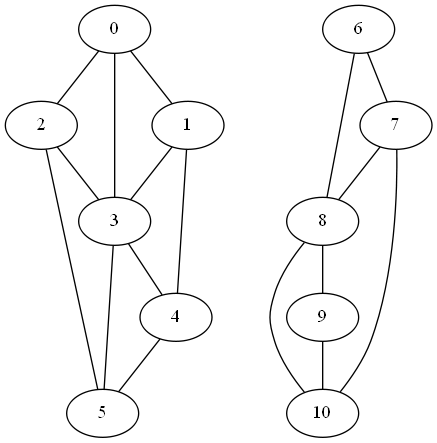
The first two eigenvalues of L are zero as expected. (Actually, when I computed them numerically, I got values around 10−15, about 15 orders of magnitude smaller than the next eigenvalue, so the first two eigenvalues are zero to the limits of floating point precision.)
Next, we add an edge between nodes 4 and 9 to form a weak link between the two clusters.
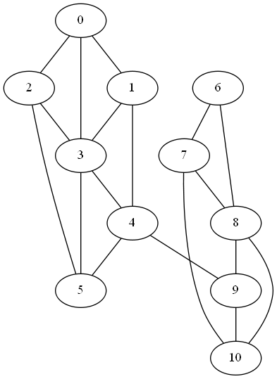
In this graph the second eigenvalue λ2 jumps to 0.2144.
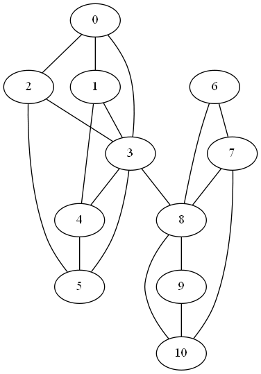
If we connect nodes 3 and 8 instead of 4 and 8, we create a stronger link between the components since nodes 3 and 8 have more connections in their respective components. Now λ2 becomes 0.2788.
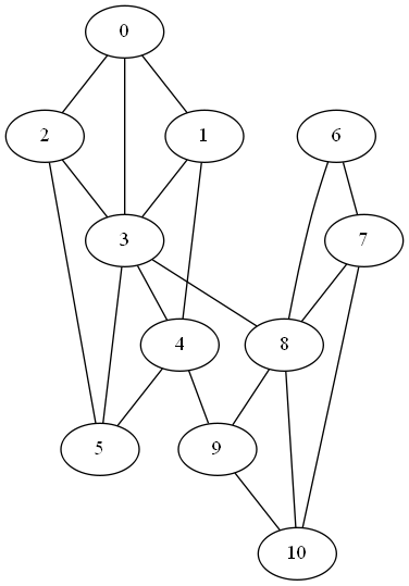
Finally if we add both, connecting nodes 4 and 9 and nodes 3 and 8, λ2 increases to 0.4989.
More graph theory
[1] To see why the smallest eigenvalue is always 0, note that v = (1, 1, 1, …, 1) is an eigenvector for 0. Multiplying the ith row of D by v picks out the degree of node i. Multiplying the ith row of A by v sums that row, which is also the degree of node i.
Can it be used in reverse (I.e. largest characteristic value) for high-influencer detection?
The explanation of why the smallest eigenvalue is always 0 is, strictly, only an explanation of why *some* eigenvalue is always 0. Why’s it the smallest? Because all the eigenvalues are non-negative. Why? Well, e.g., suppose v is an eigenvector with eigenvalue k. WLOG v1 is the largest component of v and is positive; then we have k.v1 = sum a1j.vj = d1.v1 – sum vj where d1 is the degree of vertex 1 and the sum is now over neighbours of vertex 1. And this is >= d1.v1 – sum |v1| >= 0, so k is non-negative.
(Or: apply the “Gershgorin circle theorem”. The proof-sketch above is basically the proof of the GCT specialized to this case.)
Oh, or: the eigenvalues are non-negative, because the Laplacian L is nonnegative definite, because L = Q.Qt where Qij is +-1 when there’s an edge ij (+1 for ij, -1 for ji, doesn’t matter which way around you put them) and 0 otherwise, so xt.L.x = xt.Q.Qt.x which is the inner product of Qt.x with itself and therefore nonnegative.
What does the second smallest eigenvalue tell you about the connectivity of a graph that you couldn’t already gleam from computing its vertex connectivity or edge connectivity?