Cobweb plots are a way of visualizing iterations of a function.
For a function f and a starting point x, you plot (x, f(x)) as usual. Then since f(x) will be the next value of x, you convert it to an x by drawing a horizontal line from (x, f(x)) to (f(x), f(x)). In other words, you convert the previous y value to an x value by moving to where a horizontal line intersects the line y = x. Then you go up from the new x to f applied to the new x. The Python code below makes this all explicit.
Update: I made a couple changes after this post was first published. I added the dotted line y = x to the plots, and I changed the aspect ratio from the default to 1 to make the horizontal and vertical scales the same.
    import matplotlib.pyplot as plt
    from scipy import cos, linspace

    def cobweb(f, x0, N, a=0, b=1):
        # plot the function being iterated
        t = linspace(a, b, N)
        plt.plot(t, f(t), 'k')

        # plot the dotted line y = x
        plt.plot(t, t, "k:")

        # plot the iterates
        x, y = x0, f(x0)
        for _ in range(N):
            fy = f(y)
            plt.plot([x, y], [y,  y], 'b', linewidth=1)
            plt.plot([y, y], [y, fy], 'b', linewidth=1)
            x, y = y, fy

        plt.axes().set_aspect(1)
        plt.show()
        plt.close()
The plot above was made by calling
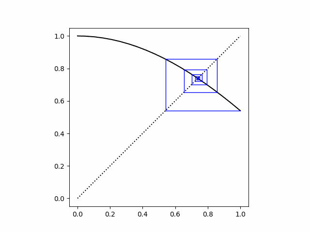
cobweb(cos, 1, 20)
to produce the cobweb plot for 20 iterations of cosine starting with x = 1. There’s one fixed point, and the cobweb plot spirals into that fixed point.
Next let’s look at several iterations of the logistic map f(x) = rx(1 − x) for differing values of r.
# one fixed point
cobweb(lambda x: 2.9*x*(1-x), 0.1, 100)
# converging to two-point attractor
cobweb(lambda x: 3.1*x*(1-x), 0.1, 100)
# starting exactly on the attractor
cobweb(lambda x: 3.1*x*(1-x), 0.558, 100)
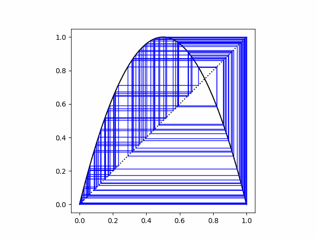
# in the chaotic region.
cobweb(lambda x: 4.0*x*(1-x), 0.1, 100)
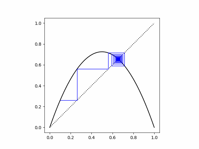
The logistic map also has one stable fixed point if r ≤ 3. In the plot below, r = 2.9.
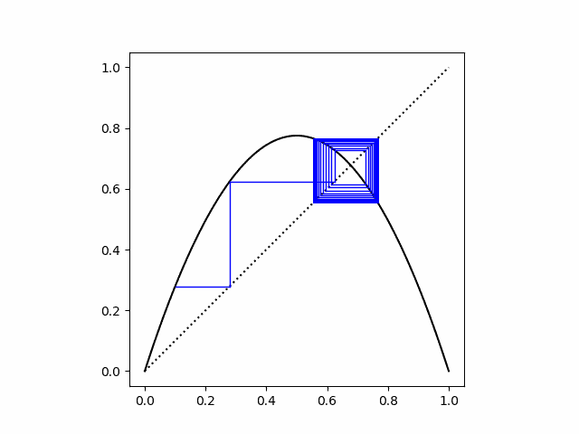
Next we set r = 3.1. We start at x = 0.1 and converge to the two attractor points.
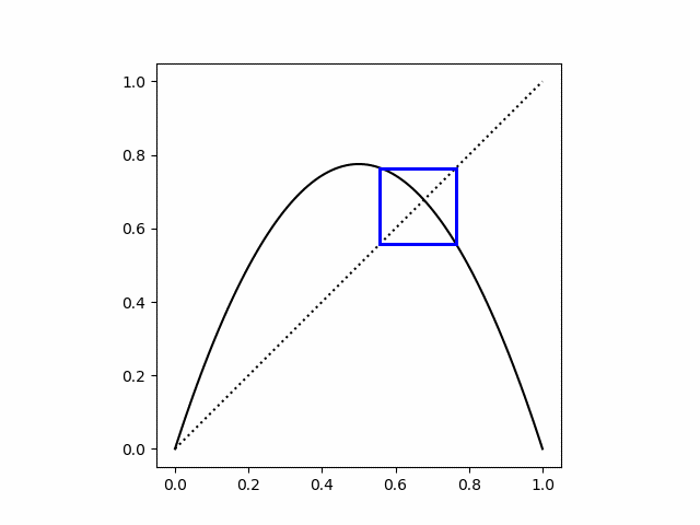
If we start exactly on one of the attractor points the cobweb plot is simply a square.
Finally, when we set r = 4 we’re in the chaotic region.
The explanation would be made more clear if at least in one of those plots the “y = x” line was also plotted (perhaps with different style, different thickness, and/or different color).
Jakub: You’re right. I changed the plots to include the diagonal line. Thanks.
Hmm, it’s easy to graphically spot a fixed point (aka 1-cycle) with this plot, and I think you can tell if it’s stable by looking at the slope there, but it’s not obvious to me how to locate a 2-cycle.
I’m thinking about moving a carpenter’s square along some fixed track, but can’t nail down the details. Any ideas?