A “rose” in mathematics is typically a curve with polar equation
r = cos(kθ)
where k is a positive integer. If k is odd, the resulting graph has k “petals” and if k is even, the plot has 2k petals.
Sometimes the term rose is generalized to the case of non-integer k. This is the sense in which I’m using the phrase “rational rose.” I’m not referring to an awful piece of software by that name [1]. This post will look at a particular rose with k = 2/3.
My previous post looked at
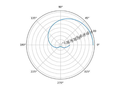
r = cos(2θ/3)
and gave the plot below.
Unlike the case where k is an integer, the petals overlap.
In this post I’d like to look at two things:
- The curvature in the figure above, and
- Differences between polar plots in Python and Mathematica
Curvature
The graph above has radius 1 since cosine ranges from −1 to 1. The curve is made of arcs that are approximately circular, with the radius of these approximating circles being roughly 1/2, sometimes bigger and sometimes smaller. So we would expect the curvature to oscillate roughly around 2. (The curvature of a circle of radius r is 1/r.)
The curvature can be computed in Mathematica as follows.
    numerator = D[x[t], {t, 1}] D[y[t], {t, 2}] -
                D[x[t], {t, 2}] D[y[t], {t, 1}]
    denominator = (D[x[t], t]^2 + D[y[t], t]^2)^(3/2)
    Simplify[numerator / denominator]
This produces

A plot shows that the curvature does indeed oscillate roughly around 2.
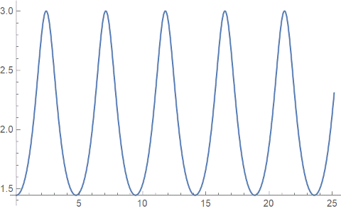
The minimum curvature is 13/9, which the curve takes on at polar coordinate (1, 0), as well as at other points. That means that the curve starts out like a circle of radius 9/13 ≈ 0.7.
The maximum curvature is 3 and occurs at the origin. There the curve is approximately a circle of radius 1/3.
Matplotlib vs Mathematica
To make the plot we’ve been focusing on, I plotted
r = cos(2θ/3)
in Mathematica, but in matplotlib I had to plot
r = |cos(2θ/3)|.
In both cases, θ runs from 0 to 8π. To highlight the differences in the way the two applications make polar plots, let’s plot over 0 to 2π with both.
Mathematica produces what you might expect.
PolarPlot[Cos[2 t/3], {t, 0, 2 Pi}]
![Mathematica plot of Cos[2 theta/3]](https://www.johndcook.com/polar_mmca.png)
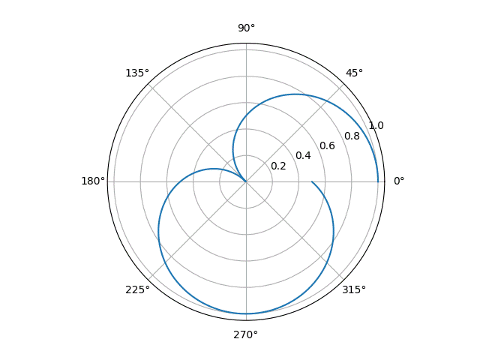
Matplotlib produces something very different. It handles negative r values by moving the point r = 0 to a circle in the middle of the plot. Notice the r-axis labels at about 22° running from −1 to 1.
    theta = linspace(0, 2*pi, 1000)
    plt.polar(theta, cos(2*theta/3))
Note also that in Mathematica, the first argument to PolarPlot is r(θ) and the second is the limits on θ. In matplotlib, the first argument is θ and the second argument is r(θ).
Note that in this particular example, taking the absolute value of the function being plotted was enough to make matplotlib act like I expected. That’s only happened true when plotted over the entire range 0 to 8π. In general you have to do more work than this. If we insert absolute value in the plot above, still plotting from 0 to 2π, we do not reproduce the Mathematca plot.
plt.polar(theta, abs(cos(2*theta/3)))
More polar coordinate posts
[1] Rational Rose was horribly buggy when I used it in the 1990s. Maybe it’s not so buggy now. But I imagine I still wouldn’t like the UML-laden style of software development it was built around.
The worst problem with Rose is that it is overpriced. Here is an alternative that is better from every standpoint: https://sparxsystems.com/
You want to code behind. Hear me now and believe me later.
Rational Rose RT was used by an infamous class in my university. We had to build an entire multiplayer game using UML and a bit of C++ in the transitions, combined with a Java Swing GUI. It was awful and had a tendency to crash and delete half your project.