I keep running into the function
f(z) = (1 − z)/(1 + z).
The most recent examples include applications to radio antennas and mental calculation. More on these applications below.
Involutions
A convenient property of our function f is that it is its own inverse, i.e. f( f(x) ) = x. The technical term for this is that f is an involution.
The first examples of involutions you might see are the maps that take x to −x or 1/x, but or function shows that more complex functions can be involutions as well. It may be the simplest involution that isn’t obviously an involution.
By the way, f is still an involution if we extend it by defining f(−1) = ∞ and f(∞) = −1. More on that in the next section.
Möbius transformations
The function above is an example of a Möbius transformation, a function of the form
(az + b)/(cz + d).
These functions seem very simple, and on the surface they are, but they have a lot of interesting and useful properties.
If you define the image of the singularity at z = −d/c to be ∞ and define the image of ∞ to be a/c, then Möbius transformations are one-to-one mappings of the extended complex plane, the complex numbers plus a point at infinity, onto itself. In fancy language, the Möbius transformations are the holomorphic automorphisms of the Riemann sphere.
More on why the extended complex plane is called a sphere here.
One nice property of Möbius transformations is that they map circles and lines to circles and lines. That is, the image of a circle is either a circle or a line, and the image of a line is either a circle or a line. You can simplify this by saying Möbius transformations map circles to circles, with the understanding that a line is a circle with infinite radius.
Electrical engineering application
Back to our particular Möbius transformation, the function at the top of the post.
I’ve been reading about antennas, and in doing so I ran across the Smith chart. It’s essentially a plot of our function f. It comes up in the context of antennas, and electrical engineering more generally, because our function f maps reflection coefficients to normalized impedance. (I don’t actually understand that sentence yet but I’d like to.)
The Smith chart was introduced as a way of computing normalized impedance graphically. That’s not necessary anymore, but the chart is still used for visualization.
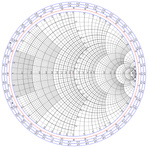
Image Wdwd, CC BY-SA 3.0, via Wikimedia Commons.
Mental calculation
It’s easy to see that
f(a/b) = (b − a)/(b + a)
and since f is an involution,
a/b = f( (b − a)/(b + a) ).
Also, a Taylor series argument shows that for small x,
f(x)n ≈ f(nx).
A terse article [1] bootstraps these two properties into a method for calculating roots. My explanation here is much longer than that of the article.
Suppose you want to mentally compute the 4th root of a/b. Multiply a/b by some number you can easily take the 4th root of until you get a number near 1. Then f of this number is small, and so the approximation above holds.
Bradbury gives the example of finding the 4th root of 15. We know the 4th root of 1/16 is 1/2, so we first try to find the 4th root of 15/16.
(15/16)1/4 = f(1/31)1/4 ≈ f(1/124) = 123/125
and so
151/4 ≈ 2 × 123/125
where the factor of 2 comes from the 4th root of 16. The approximation is correct to four decimal places.
Bradbury also gives the example of computing the cube root of 15. The first step is to multiply by the cube of some fraction in order to get a number near 1. He chooses (2/5)3 = 8/125, and so we start with
15 × 8/125 = 24/25.
Then our calculation is
(24/25)1/3 = f(1/49)1/3 ≈ f(1/147) = 73/74
and so
151/3 ≈ (5/2) × 73/74 = 365/148
which is correct to 5 decimal places.
Update: See applications of this transform to mentally compute logarithms.
[1] Extracting roots by mental methods. Robert John Bradbury, The Mathematical Gazette, Vol. 82, No. 493 (Mar., 1998), p. 76.
That’s clever, but how are you supposed to find an appropriate nth power to multiply x?
In ancient days before microcomputers ruled the Earth and 32K was seen as a huge amount of memory, I worked as an EE in the defense industry. Smith charts, nomograms, and of course the noble slide rule were all part of the engineer’s toolkit. Today I’m a devoted Mathematica user; yet, there were advantages to the old tools which could give an intuitive and broader view of a computation. In my classes I always try to recapture some of those benefits through Fermi questions, interactive graphics, simple simulations, and similar approaches. Surprisingly, one field that still makes extensive use of nomograms is medicine—which is interesting and perhaps a bit scary.
@Aaron: Good question. So you start with x and you want to find y such that xy is approximately 1. So y is approximately 1/x. You want to find a ratio of nth powers that approximately equals 1/x.
It’s saying that you have to start with an approximate nth root of (the reciprocal of) x, which sounds circular, but it’s not. It’s actually iterative refinement. You start with a rough approximation and produce a better approximation.
In the case of the 4th root of 15, you can start by observing that the 4th root is near 2. So (1/2)^4 is an appropriate y. I suppose you could take the output of Bradury’s trick and use it again to get a very accurate approximation.
In the second example, it’s not so clear how to find a ratio of cubes that approximately equals 1/15, and so (2/5)^2 may seem less motivated than the choice of 1/16 in the first example.
@Robert: I think it would be useful to make students use slide rules etc for a week. Maybe one week a year.
In the first occurrence in Smith’s chart section, you used “inductance” instead of “impedance”. By the way, since f is an involution, the chart can be useful also the other way round.
An application of this function in linear algebra is the Cayley Transform [1], which maps between skew-symmetric matrices and orthogonal matrices. By the spectral mapping theorem this corresponds to a mapping of the eigenvalues in the complex plane by the original function. The mapping goes between a half-plane and a disc. Another mapping that does this is the exponential function. A nice property of the Cayley Transform is that it only requires one linear solve, whereas taking the exponential of a matrix is a lot more involved.
[1] https://en.wikipedia.org/wiki/Cayley_transform
The reflection coefficient ([1]) “is a parameter that describes how much of a wave is reflected by an impedance discontinuity in the transmission medium”. It is defined by the formula:
Gamma = (ZL-Z0)/(ZL+ZO)
Where “ZL” is the impedance of your load (for instance, your phone being charged) and ZO is the impedance of the line (the impedance of the charging cable).
For circuits with low frequencies the impedance of the line (ZO) is so small in comparison to ZL that you can neglect it, so your reflection coefficient is one, and all the power is being transmitted to the load.
For circuits with high frequencies the impedance of the line is usually not negibible in comparison with the load, and has to be taken into account. For instance, the coaxial cable that connects an antenna to your TV set. You want to make sure that the reflection coefficient is one, so all antenna signal is sent to your TV, so you usually have to add some specific extra impedances in the line to correct the mismatched impedances. You use the Smith chart to compute these impedances, and then you connect a “matching impedance” to ensure that the reflection coefficient is close to one. These “extra impedances” are usually called “stubs” [2].
The “normalized impedance” is just dividing everything by the line impedance, so the “normalized reflection coefficient” is:
Gamma/ZO = (ZL/ZO – 1) / (ZL/ZO + 1)
This is, you just think the “line impedance” is one, and you correct the load impedance by dividing it by the line impedance (ZL/ZO).
The Smith chart is just this function (a plot of the “normalized reflection coefficient with line impedance equal to one”), and can be used in all transmission lines no matter what the line impedance is, but you’ll have to remember to multiply back by ZO in order to have a proper real value for your transmission line.
[1]
https://en.wikipedia.org/wiki/Reflection_coefficient#Relation_to_load_impedance
[2]
https://en.wikipedia.org/wiki/Stub_(electronics)