Nonlinear phase portrait

I was reading through Michael Trott’s Mathematica Guidebook for Programming and ran across the following plot.

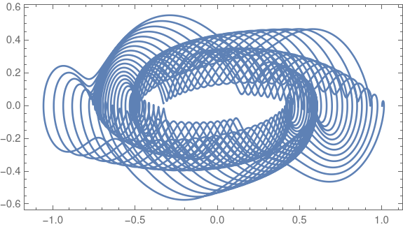
I find the image aesthetically interesting. I also find it interesting that the image is the phase portrait of a differential equation whose solution doesn’t look that interesting. That is, the plot of (x(t), x ‘(t)) is much more visually interesting than the plot of x(t).

The differential equation whose phase portrait is plotted above is

with initial position 1 and initial velocity 0. It’s a familiar damped, driven harmonic oscillator, except the equation is nonlinear because the derivative term is cubed.

Here’s a plot of the solution as a function of time.

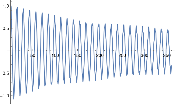
The solution basically looks like the solution of the linear case, except the solutions are more jagged near the local maxima and minima. In fact, the plot looks so jagged that I wondered whether this was an artifact of needing more plotting points. But adding more points didn’t make much difference. Interestingly, although this plot looks jagged, the phase portrait is smooth.

I produced the phase portrait by copying Trott’s code and making a couple small modifications.

    sol = NDSolve[{(*differential equation*)
        x''[t] + 1/20 x'[t]^3 + 1/5 x[t] == 
        1/3 Cos[E t],(*initial conditions*)x[0] == 1, x'[0] == 0}, 
        x, {t, 0, 360}, MaxSteps -> Infinity]

    ParametricPlot[Evaluate[{x[t], x'[t]} /. sol], {t, 0, 360}, 
        Frame -> True, Axes -> False, PlotPoints -> 3600]

Apparently the syntax of NDSolve has changed slightly since Trott’s book was published in 2004. The argument x in the code above was written x[t] in Trott’s original code and this did not work in the current version of Mathematica. I also simplified the call to ParametricPlot slightly, though the original code would work.