The equation of motion for a pendulum is the differential equation

where g is the acceleration due to gravity and ℓ is the length of the pendulum. When this is presented in an introductory physics class, the instructor will immediately say something like “we’re only interested in the case where θ is small, so we can rewrite the equation as

Questions
This raises a lot of questions, or at least it should.
- Why not leave sin θ alone?
- What justifies replacing sin θ with just θ?
- How small does θ have to be for this to be OK?
- How do the solutions to the exact and approximate equations differ?
First, sine is a nonlinear function, making the differential equation nonlinear. The nonlinear pendulum equation cannot be solved using mathematics that students in an introductory physics class have seen. There is a closed-form solution, but only if you extend “closed-form” to mean more than the elementary functions a student would see in a calculus class.
Second, the approximation is justified because sin θ ≈ θ when θ is small. That’s true, but it’s kinda subtle. Here’s a post unpacking that.
The third question doesn’t have a simple answer, though simple answers are often given. An instructor could make up an answer on the spot and say “less than 10 degrees” or something like that. A more thorough answer requires answering the fourth question.
I address how nonlinear affects the solutions in a post a couple years ago. This post will expand a bit on that post.
Longer period
The primary difference between the nonlinear and linear pendulum equations is that the solutions to the nonlinear equation have longer periods. The solution to the linear equation is a cosine. Solving the equation determines the frequency, amplitude, and phase shift of the cosine, but qualitatively it’s just a cosine. The solution to the corresponding nonlinear equation, with sin θ rather than θ, is not exactly a cosine, but it looks a lot like a cosine, only the period is a little longer [1].
OK, the nonlinear pendulum has a longer period, but how much longer? The period is increased by a factor f(θ0) where θ0 is the initial displacement.
You can find the exact answer in my earlier post. The exact answer depends on a special function called the “complete elliptic integral of the first kind,” but to a good approximation

The earlier post compares this approximation to the exact function.
Linear solution with adjusted period
Since the nonlinear pendulum equation is roughly the same as the linear equation with a longer period, you can approximate the solution to the nonlinear equation by solving the linear equation but increasing the period. How good is that approximation?
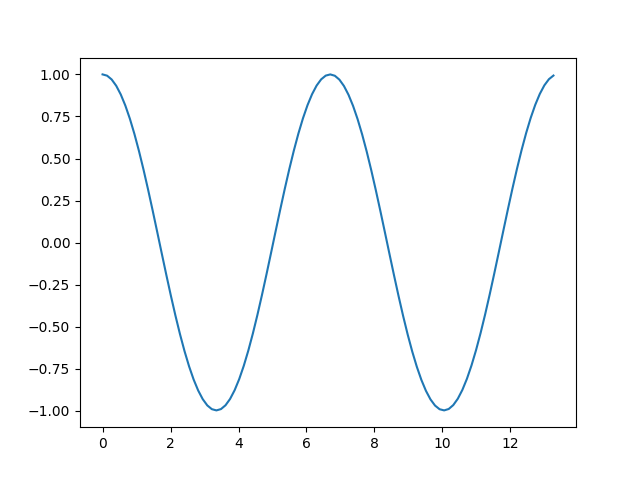
Let’s do an example with θ0 = 60° = π/3 radians. Then sin θ0 = 0.866 but θ0, in radians, is 1.047, so we definitely can’t say sin θ0 is approximately θ0. To make things simple, let’s set ℓ = g. Also, assume the pendulum starts from rest, i.e. θ'(0) = 0.
Here’s a plot of the solutions to the nonlinear and linear equations.
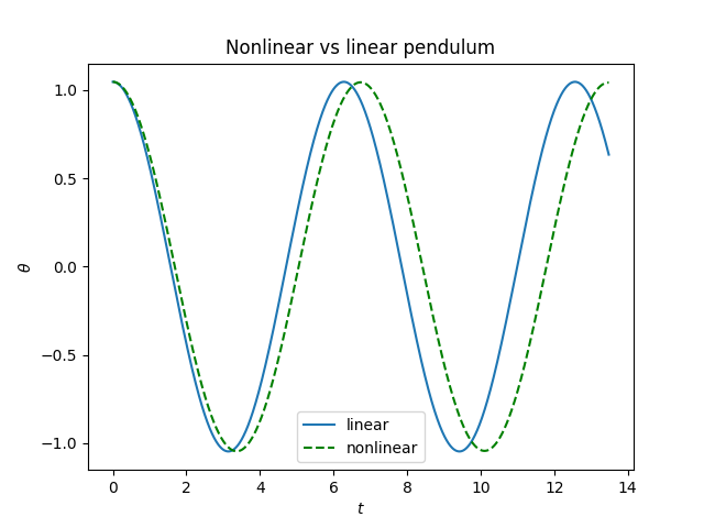
Obviously the solution to the nonlinear equation has a longer period. In fact it’s 7.32% longer. (The approximation above would have estimated 7.46%.)
Here’s a plot comparing the solution of the nonlinear equation and the solution to the linear equations with period stretched by 7.32%.
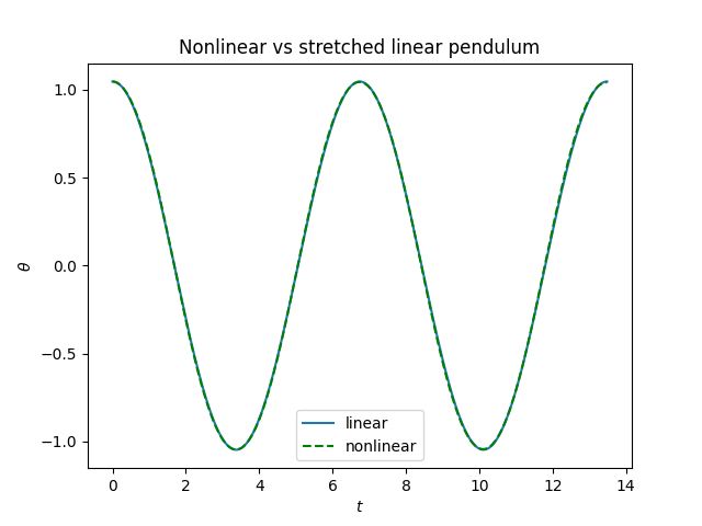
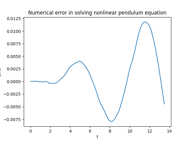
The solutions differ by less than the width of the plotting line, so it’s too small to see. But we can see there’s a difference when we subtract the two solutions.
Here’s a plot of the solutions to the nonlinear and linear equations.
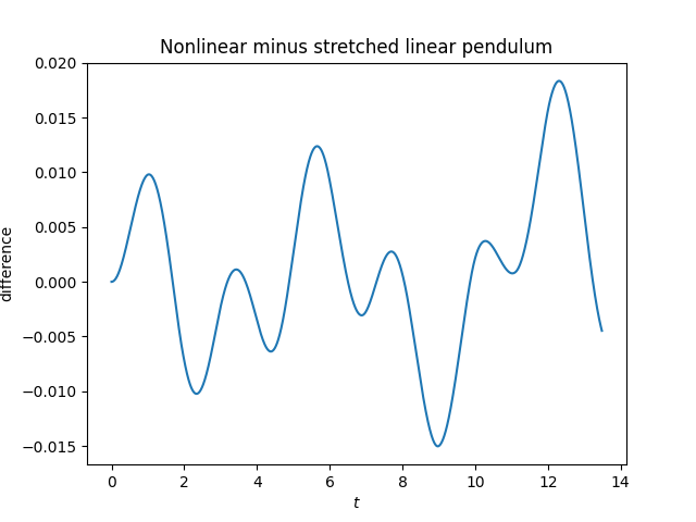
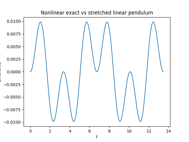
Update: The plot above is misleading. Part of what it shows is numerical error from solving the pendulum equation. When we redo the plot using the exact solution the error is about half as large. And the error is periodic, as we’d expect. See this post for more on the exact solution using Jacobi functions and the differential equation solver that was used to make the original plot.
Related posts
[1] The period of a pendulum depends on its length ℓ, and so we can think of the nonlinear term effectively replacing ℓ by a longer effective length ℓeff.