The following 2D bifurcation diagram is famous. You’ve probably seen it elsewhere.
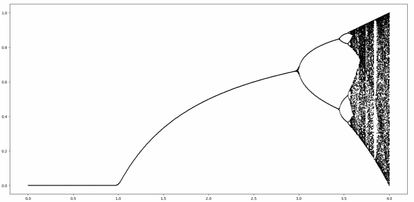
If you have seen it, you probably know that it has something to do with chaos, iterated functions, fractals, and all that. If you’d like to read in more detail about what exactly the plot means, see this post.
I was reading Michael Trott’s Mathematica Guidebook for Numerics and ran across a 3D version of the above diagram. I’d never seen that before. He plots the iterations of the system
x ← a − y(β x + (1 − β) y)
y ←x + y²/100
The following plot is for β = 1/4 using the code included in the book. (I changed the parameter α in the book to β because the visual similarity between a and α was a little confusing.)
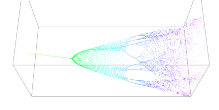
Trott cites four papers regarding this iteration. I looked at a couple of the papers, and they contain similar systems but aren’t quite the same. Maybe his example is a sort of synthesis of the examples he found in the literature.
Related posts: More on dynamical systems
There’s also a cool way to make a 3d bifurcation diagram involving the Mandlebrot set, seen at 6:40 in this video: https://www.youtube.com/watch?v=ovJcsL7vyrk&t=400s.
Great post,
This diagram is also used when applying Principle Component Analysis to managing the Cost, Schedule, and Technical Performance of programs in our Aerospace & Defense domain.
The “second” branch happens when during the modeling of Analysis or Alternatives when the path on the left of that second branch produces unacceptable or unanticipated outcomes – “our prototype crashed on the test range! What Plan B?”