The function
f(x) = 1/(1 + x²)
is commonly used as an example to disprove a couple things students might be lead to believe. This post will show how the logistic function
g(x) = exp(x)/(1 + exp(x))
could be used in the same contexts. This shows that f(x) is not an isolated example, and the phenomena that it illustrates are not so rare.
Radius of convergence
One thing that f is commonly used to illustrate is that the power series of a function can have a finite radius even though the function is infinitely differentiable with no apparent singularities. I say “apparent” because the function f has no singularities as long as you think of it as a function of a real variable. When you think of it as a function of a complex variable, it has singularities at ±i.
The radius of convergence of a function is something of a mystery if you only look along the real line. (You may see “interval” of convergence in textbooks. I’m tipping my hand by using the word “radius.”) If a function has a power series in the neighborhood of a point, the radius of convergence for that series is determined by the distance to the nearest singularity in the complex plane, even if you’re only interested in evaluating the series at real numbers. For example,
f(x) = 1 − x2 + x4 − x6 + ⋯
The series converges for |x| < 1. If you stick in an x outside this range, say x = 3, you get the absurd [1] equation
1/10 = 1 − 9 + 81 − 729 + ⋯
The logistic function g also has a finite radius of convergence, even though the function is smooth everywhere along the real line. It has a singularity in the complex plane when exp(x) = −1, which happens at odd multiples of πi. So the power series for g centered at 0 has a radius of π, because that’s the distance from 0 to the nearest singularity of g.
Runge phenomenon
Carl David Tolmé Runge, best known for the Runge-Kutta algorithm, discovered that interpolating a function at more points may give worse results. In fact, the maximum interpolation error can go to infinity as the number of interpolation points increases. This is true for the Cauchy function f above, but also for the logistic function g. As before, the explanation lies in the complex plane.
Runge’s proved that trouble occurs when interpolating over the segment [−1, 1] at evenly-spaced points [2] if the function being interpolated has a singularity inside a certain region in the complex plane. See [3] for details.When we interpolate
g(x) = exp(ax)/(1 + exp(ax))
we can see the Runge phenomenon if a is large enough and if we interpolate at enough points. In the Mathematica code below, we use a = 10 and interpolate at 22 points.
    g[x_, a_] := Exp[a x]/(1 + Exp[a x])
    p[x_, a_, n_] :=  InterpolatingPolynomial[
        Table[{s, g[s, a]}, {s, -1.0, 1.0, 2/n}], x]
    Plot[{g[x, 10], p[x, 10, 22]}, {x, -1, 1}]
Here’s the plot.
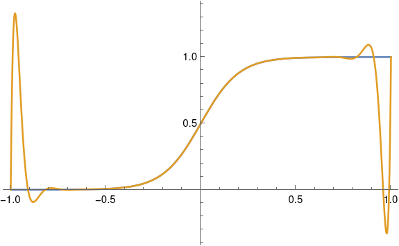
Note that we get a good fit over much of the interval; the two curves agree to within the thickness of a plotting line. But we get huge error near the ends. There we can see the flat blue line sticking out.
Obviously approximating a nearly flat function with a huge spike is undesirable. But even if the spikes were only small ripples, this could still be a problem. In some contexts, approximating a monotone function by a function that is not monotone can be unacceptable, even if the approximation error is small. More on that here.
Related posts
[1] You may have seen the “equation”
1 + 2 + 3 + ⋯ = −1/12.
This and the equation
1 − 9 + 81 − 729 + ⋯ = 1/10
are both abuses of notation with a common explanation. In both cases, you start with a power series for a function that is valid in some limited region. The left side of the equation evaluates that series where the series does not converge, and the right side of the equation evaluates an analytic continuation of the function at that same point. In the first example, the function is the Riemann zeta function ζ(s) which is defined by
![]()
for s with real part larger than 1. The series converges when the real part of s is larger than 1. The example evaluates the series at −1. The zeta function can be extended to a region containing −1, and there it has the value −1/12.
[2] You can avoid the problem by not using evenly spaced points, e.g. by using Chebyshev interpolation.
[3] Approximation Theory and Approximation Practice by Lloyd N. Trefethen