Approximating the range of normal samples

On Monday I wrote a blog post that showed you can estimate the standard deviation of a set of data by first computing its range and then multiplying by a constant. The advantage is that it’s easy to compute a range, but computing a standard deviation in your head would be tedious to say the least.

The problem, or the interesting part, depending on your perspective, is the constants d_n you have to multiply the range by.

Yesterday before work I wrote a blog post about a proposed approximation d_n and yesterday after work I wrote a post on the exact values.

There have been a couple suggestions in the comments for how to approximate d_n, namely √n and log n. There’s merit to both over different ranges.

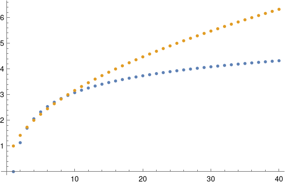
Here’s a plot of d_n and √n. You can see that √n is an excellent approximation to d_n for n between 3 and 10: the gold and blue dots overlap. But for larger n, √n grows too fast. It keeps going while d_n sorta plateaus.

For larger n, log n is a better approximation to d_n. When n = 100, the square root approximation is about twice the exact value, but the log approximation if fairly close. The error in the log approximation seems to be decreasing slowly, maybe going to zero or to a small constant.

There are more accurate approximations out there. In 1958, Gunnar Blom [1] published the approximation

You can get good results for moderately large n by taking α = 0.375, and you can get even better results by adjusting α over various ranges of r and n.

As I wrote last night, E(r, n) is the expected value of the rth order statistic from a sample of size n, Φ is the CDF of a standard normal, and d_n = 2 E(n, n).

We can implement Blom’s approximation with the following Mathematica code.

    PhiInv[x_] := Sqrt[2] InverseErf[2 x - 1]
    alpha = 0.375
    Blom[n_] := -2 PhiInv[(1 - alpha)/(n - 2 alpha + 1)]

If we plot d_n and Blom’s approximation on the same plot, we won’t be able to tell them apart: the dots overlap. We can plot the difference between the two values with

    ListPlot[Table[d[n] - Blom[n], {n, 1, 100}]]

and get the following graph.

There have been more accurate approximations developed since 1958, but that’s as far as I want to go down this rabbit hole for now.

Update: I just noticed a comment on the first post in this series. Ashley Kanter’s approximation was supposed to be

3 (log₁₀ n) ^0.75

and not

3 log₁₀ (n^0.75)

The former is quite good, with a an error comparable to Blom’s method. Here’s a plot of the error:

 

[1] Gunnar Blom (1958). Statistical Estimates and Transformed Beta-Variables. John Wiley and Sons Inc.