Order statistics for normal distributions

The last couple posts have touched on order statistics for normal random variables. I wrote the posts quickly and didn’t go into much detail, and more detail would be useful.

Given two integers n ≥ r ≥ 1, define E(r, n) to be the rth order statistic of n samples from standard normal random variables. That is, if we were to take n samples and then sort them in increasing order, the expected value of the rth sample is E(r, n).

We can compute E(r, n) exactly by

$E(r, n) = \frac{n!}{(r-1)!\, (n-r)!} \int_{-\infty}^\infty x (1 - \Phi(x))^{r-1}\,\Phi(x)^{n-r}\, \phi(x) \, dx$

where φ and Φ are the PDF and CDF of a standard normal random variable respectively. We can numerically evaluate E(r, n) by numerically evaluating its defining integral.

The previous posts have used

d_n = E(n, n) – E(1, n) = 2 E(n, n).

The second equality above follows by symmetry.

We can compute d_n in Mathematica as follows.

    Phi[x_] := (1 + Erf[x/Sqrt[2]])/2    
    phi[x_] := Exp[-x^2/2]/Sqrt[2 Pi]
    d[n_] := 2 n NIntegrate[
        x Phi[x]^(n - 1) phi[x], {x, -Infinity, Infinity}]

And we can reproduce the table here by

    Table[1/d[n], {n, 2, 10}]

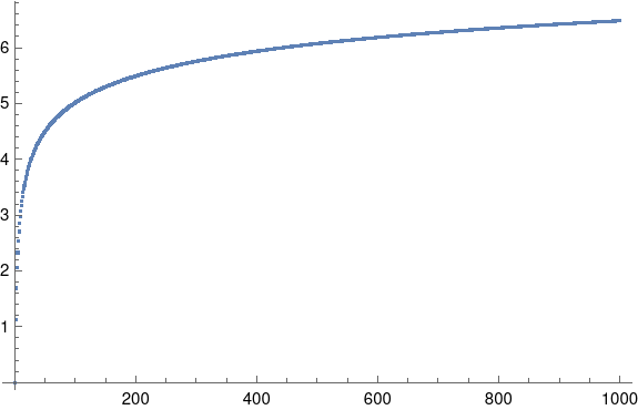
Finally, we can see how d_n behaves for large n by calling

    ListPlot[Table[d[n], {n, 1, 1000}]]

to produce the following graph.

See the next post for approximations to d_n.