Iterated golden rectangles in detail

I’ve seen the illustration of nesting golden rectangles many times, but I’ve never seen a presentation go into much detail. This post will go into more detail than usual, including Python code.

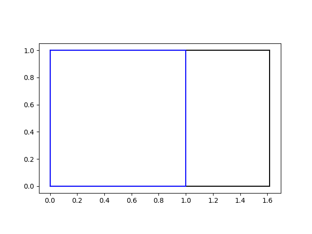
Start with a golden rectangle in landscape mode. We’ll plot our rectangle with the lower left corner at the origin and the upper right corner at (φ, 1) where φ is the golden ratio. No imaging cutting off the largest square you can on the left side, shown in blue.

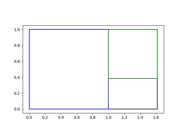
Next, focus on the remaining rectangle and imagine cutting off the square on top, shown in green.

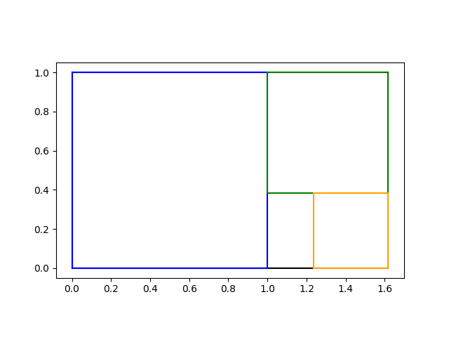
Now focus on the remaining rectangle and imagine cutting off the square on the right, shown in orange.

Finally, focus on the remaining rectangle and imagine cutting off the square on bottom, shown in red.

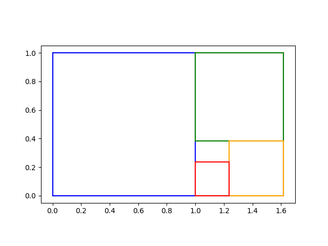
So we’ve cut off left, top, right, and bottom. We’re left with a rectangle with one side of each color above. We could repeat the process above on this rectangle, cutting off left, top, right, and bottom, and so on ad infinitum.

Where does this process end in the limit? Draw two diagonal lines as shown below.

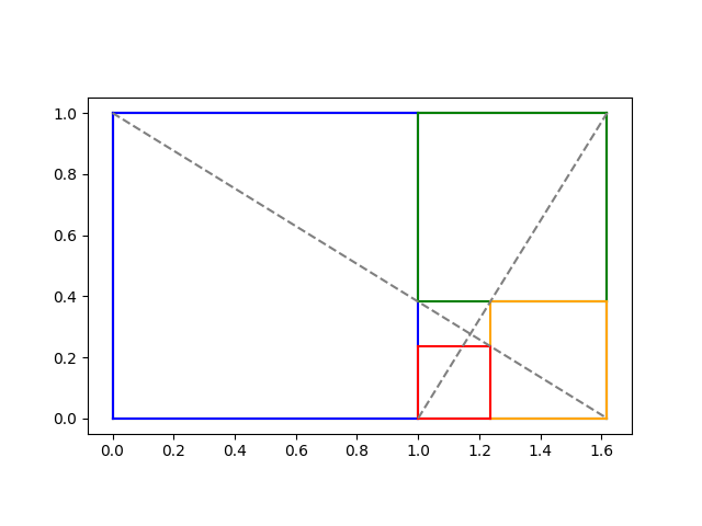
Note that these diagonals cut the innermost rectangle in the same way as the outermost rectangle. So every time we repeat the four steps above, we will always have two diagonals that intersect in the same place. So the limit of the process converges on the point that is the intersection of the two diagonal lines.

The two diagonals lines have equations

y = -(1/φ)x + 1

and

y = φx – φ

and so we can calculate their intersection to be at

x₀ = (2φ + 1)/(φ + 2)

and

y₀ = 1/(φ + 2).

So the construction process, in the limit, converges to the point (x₀, y₀) where the diagonals cross.

Here’s Python code to product the final plot above.

    import numpy as np
    import matplotlib.pyplot as plt
    
    phi = (1 + 5**0.5)/2
    
    def plotrect(lowerleft, upperright, color):
        x0, y0 = lowerleft
        x1, y1 = upperright
        plt.plot([x0, x1], [y0, y0], c=color)
        plt.plot([x0, x1], [y1, y1], c=color)
        plt.plot([x0, x0], [y0, y1], c=color)
        plt.plot([x1, x1], [y0, y1], c=color)
    
    plt.gca().set_aspect("equal")   
 
    plotrect((0, 0), (phi, 1), "black")
    plotrect((0, 0), (1, 1), "blue")
    plotrect((1, 2-phi), (phi, 1), "green")
    plotrect((2*phi - 2,0), (phi, 2-phi), "orange")
    plotrect((1,0), (2*phi-2,2*phi-3), "red")
    plt.plot([0, phi], [1, 0], "--", color="gray")
    plt.plot([1, phi], [0, 1], "--", color="gray")
    plt.savefig("golden_rect5.png")

I intend to find the equation of the spiral that touches two corners of each square in the next post.