Logarithmic spiral

I’ve seen an image similar to the following many times, but I don’t recall any source going into detail regarding how the spiral is constructed. This post will do just that.

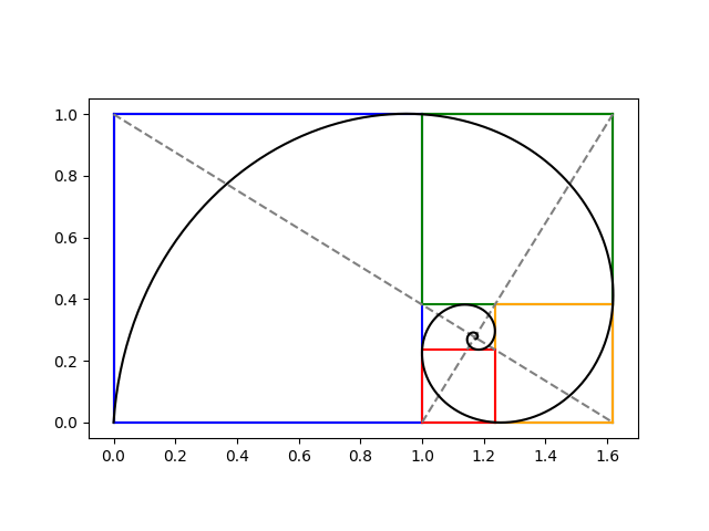
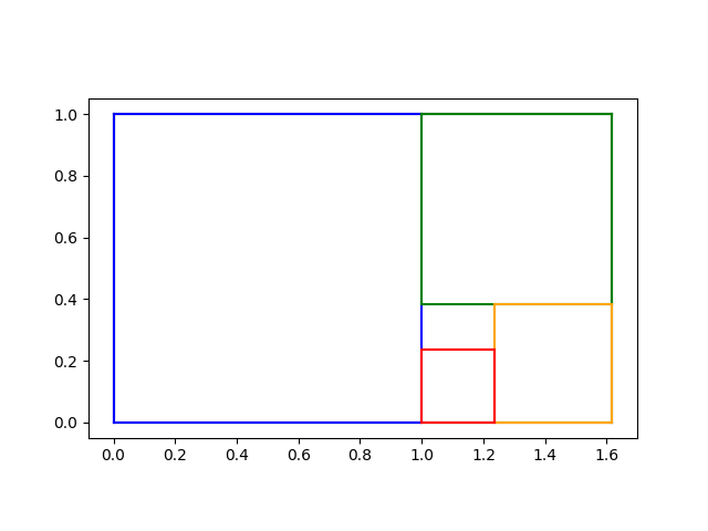
The previous post constructed iterated golden rectangles. We start with a golden rectangle and imagine chopping of first the blue, then the green, then the orange, and then the red square. We could continue this process on the inner most rectangle, over and over.

At this point, many sources would say “Hey look! We can draw a spiral that goes through two corners of each square” without explicitly stating an equation for the spiral. We’ll find spiral, making everything explicit.

In the previous post we showed how to find the limit of the iterative process at the intersection of the two diagonal lines below.

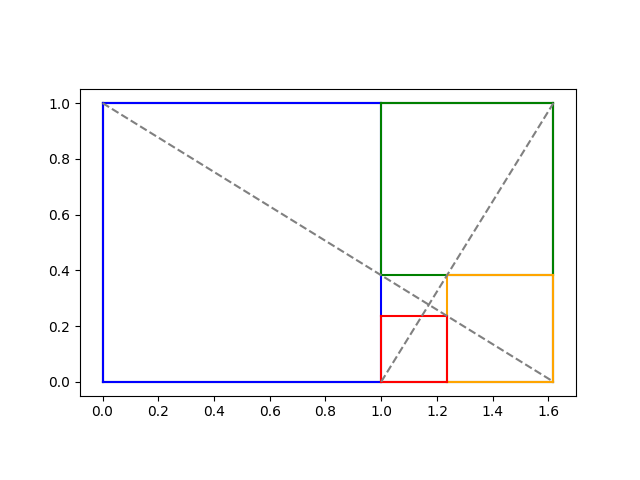
We showed that the intersection is at

x₀ = (2φ + 1)/(φ + 2)

and

y₀ = 1/(φ + 2).

Logarithmic spirals

A logarithmic spiral centered at the origin has the polar equation

r(θ) = a exp(kθ)

for some constants a and k. Our spiral will be such a spiral shifted to center at (x₀, y₀).

Imagine a spiral going from the lower left to the top left of the blue square, then to the top left of the green square, then to the top right of the orange square etc., passing through two corners of every square. Every time θ goes through a quarter turn, i.e. π/2 radians, our rectangles get smaller by a factor of φ. We can use this to solve for k because

a exp(k(θ + π/2)) = φ a exp(kθ)

and so

exp(kπ/2) = φ

and

k = 2log(φ) / π.

To summarize what we know so far, if we shift our spiral to the origin, it has equation in polar form

r(θ) = a exp(kθ)

where we now know k but don’t yet know a.

Finding θ and a

To get our actual spiral, we have to shift the origin to (x₀, y₀) which we have calculated above. Converting from polar to rectangular coordinates so we can do the shift, we have

x(θ) = x₀ + a exp(kθ) cos(θ)

y(θ) = y₀ + a exp(kθ) sin(θ)

We can find the parameter a by knowing that our spiral passes through the origin, the bottom left corner in the plots above. At what value of θ does the curve go through the origin? We have a choice; values of θ that differ by multiples of 2π will give different values of a.

The angle θ is the angle made by the line connecting (0, 0) to (x₀, y₀). We can find θ via

θ₀ = atan2(-y₀, –x₀).

Here’s Python code to find θ₀:

    import numpy as np

    phi = (1 + 5**0.5)/2
    y0 = 1/(2+phi)
    x0 = (2*phi + 1)*y0
    theta0 = np.arctan2(-y0, -x0)

Then we solve for a from the equation x(θ₀) = 0.

    k = 2*np.log(phi)/np.pi
    a = -x0 / (np.exp(k*theta0)*np.cos(theta0)))

Plots

Now we have all the parameters we need to define our logarithmic spiral. The following code draws our logarithmic spiral on top of the plot of the rectangles.

    t = np.linspace(-20, theta0, 1000)
    def x(t): return x0 + a*np.exp(k*t)*np.cos(t)
    def y(t): return y0 + a*np.exp(k*t)*np.sin(t)
    plt.plot(x(t), y(t), "k-")

The result is the image at the top of the post.