This post will give examples of three similar diagrams that occur in three dissimilar areas: design of experiments, finite difference methods for PDEs, and numerical integration.
Central Composite Design (CCD)
The most popular design for fitting a second-order response surface is the central composite design or CCD. When there are two factors being tested, the combinations of the two factors are chosen according to the following diagram, with the value at the center being used for several replications, say four.
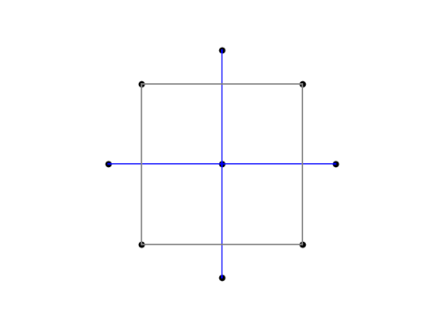
The variables are coded so that the corners of the square have both coordinates equal to ±1. The points outside the square, the so-called axial points, have one coordinate equal to 0 and another equal to ±√2.
Finite difference method
The star-like arrangement of points with the middle being weighted more heavily is reminiscent of the five-point finite difference template for the Laplacian. Notice that the center point is weighted by a factor of −4.
![]()
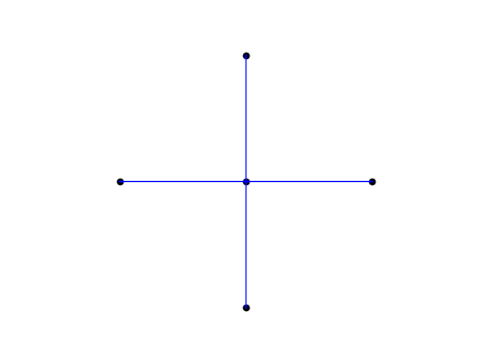
In the finite difference method, this pattern of grid points carries over to a pattern of matrix coefficients.
Integrating over a disk
The CCD grid looks even more like a numerical integration pattern for a function f defined over a disk of radius h. See A&S equation 25.4.61.
![]()
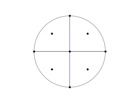
The center of the circle has weight w = 1/6. The four points on the circle are located at (±h, 0) and (0, ±h) and have weight w = 1/24. The remaining points are located at (±h/2, ±h/2) and have weight w = 1/6.