Yesterday Terence Tao published a blog post on bounds for the Poisson probability distribution. Specifically, he wrote about Bennett’s inequalities and a refinement that he developed or at least made explicit. Tao writes
This observation is not difficult and is implicitly in the literature … I was not able to find a clean version of this statement in the literature, so I am placing it here on my blog.
Bennett’s inequalities say that for a Poisson random variable X with mean λ,
for u ≥ 0 and
for -1 < u ≤ 0 where
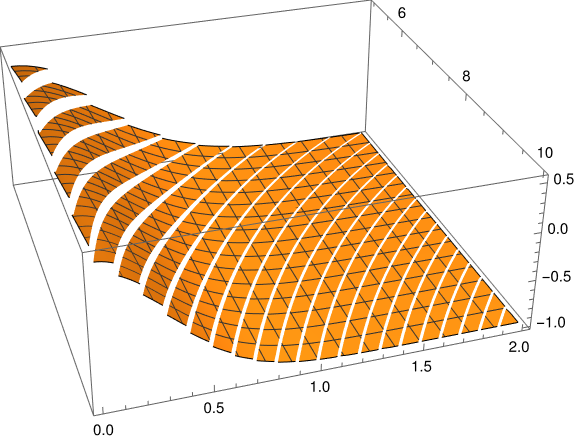
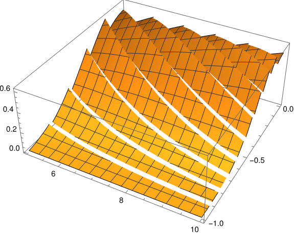
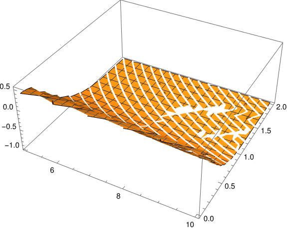
I wanted to visualize how tight Bennett’s bounds are and got some interesting images due to the discrete nature of the Poisson distribution.
Here’s a plot of how tight the right-tail estimate is, the gap between the two sides of the first inequality above.

Here u ranges from 0 to 2 along the front edge of the graphic and λ ranges from 5 to 10.
And here’s a plot of how tight the left-tail estimate is, the gap between the two sides of the second inequality above.

Mathematica tweaking
The latter image was easy to make, but the first image required a couple adjustments: the image had holes in it, and the view point was awkward.

I fixed the holes in the plot by adding the option PlotPoints->50 to make the sampling finer. I fixed the view point by grabbing the image and rotating it until I thought it looked better. I could have saved the rotated image directly, but I was curious how to do this with the Export command. To do this I needed to specify the ViewPoint explicitly in the plotting command, but I didn’t know how to get the value of ViewPoint that’s I’d implicitly found via my mouse. A comment on the Mathematica Stack Exchange site told me what I needed to know.
Simply edit the output cell and wrap Options[…, ViewPoint] around the already rotated output. The graphics should be in the place of …. ViewVertical may also change during rotating, as well as some other parameters.
