This post will reproduce a three plots from a paper of Hénon on dynamical systems from 1969 [1].
Let α be a constant, and pick some starting point in the plane, (x0, y0), then update x and y according to
xn+1 = xn cos α − (yn − xn²) sin α
yn+1 = xn sin α + (yn − xn²) cos α
When I tried out Hénon’s system for random starting points, I didn’t get plots that were as interesting as those in the original paper. Hénon clearly did a lot of experiments to produce the plots chosen for his paper. Because his system is chaotic, small changes to the initial conditions can make enormous differences to the resulting plots.
Hénon lists the starting points used for each plot, and the number of iterations for each. I imagine the number of iterations was chosen in order to stop when points wandered too far from the origin. Even so, I ran into some overflow problems.
I suspect the original calculations were carried out using single precision (32-bit) floating point numbers, while my calculations were carried out with double precision (64-bit) floating point numbers [2]. Since the system is chaotic, this minor difference in the least significant bits could make a difference.
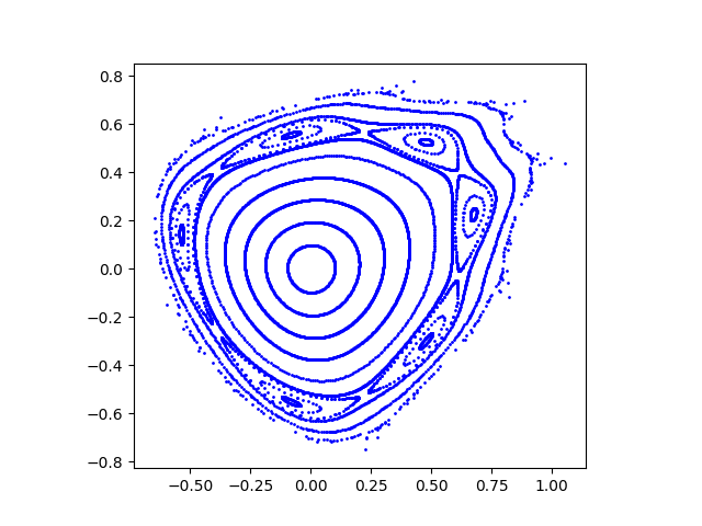
Here is my reproduction of Hénon’s Figure 4:
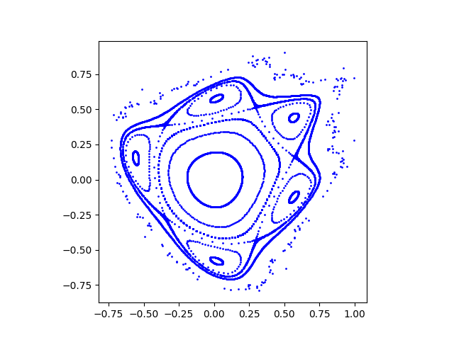
Here is my reproduction of Figure 5:
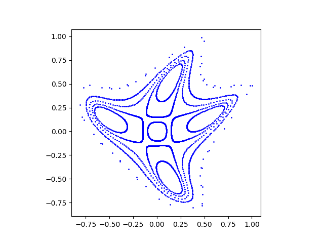
And finally Figure 7:
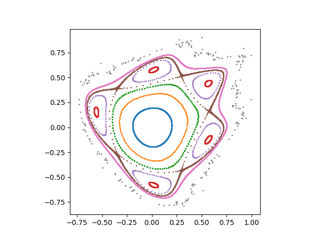
Update: You could use colors to distinguish the trajectories of different starting points. Here’s a color version of Figure 5:
Related posts
For more posts like this, see Dynamical systems & chaos.
Python code
Here is the code that produced the plots. The data starting points and number of iterations were taken from Table 1 of [1].
import matplotlib.pyplot as plt

# Hénon's dynamical system
# M. Hénon. Numerical study of squadratic area-preserving mappings. Quarterly of Applied Mathematics. October 1969 pp. 291--312

def makeplot(c, data):
    s = (1 - c*c)**0.5
    for d in data:
        x, y, n = d
        for _ in range(n):
            if abs(x) < 1 and abs(y) < 1:
                x, y = x*c - (y - x**2)*s, x*s + (y - x**2)*c
                plt.scatter(x, y, s=1, color='b')
    plt.gca().set_aspect("equal")
    plt.show()

fig4 = [
    [0.1,   0,    200],
    [0.2,   0,    360],
    [0.3,   0,    840],
    [0.4,   0,    871],
    [0.5,   0,    327],
    [0.58,  0,   1164],
    [0.61,  0,   1000],
    [0.63,  0.2,  180],
    [0.66,  0.22, 500],
    [0.66,  0,    694],
    [0.73,  0,    681],
    [0.795, 0,    657],
]

makeplot(0.4, fig4)

fig5 = [
    [0.2,   0,    651],
    [0.35,  0,    187],
    [0.44,  0,   1000],
    [0.60, -0.1, 1000],
    [0.68,  0,    250],
    [0.718, 0,   3000],
    [0.75,  0,   1554],
    [0.82,  0,    233],
]

makeplot(0.24, fig5)


fig7 = [
    [0.1, 0, 182],
    [0.15, 0, 1500],
    [0.35, 0, 560],
    [0.54, 0, 210],
    [0.59, 0, 437],
    [0.68, 0, 157],
]

makeplot(-0.01, fig7, "fig7.png")
[1] Michel Hénon. Numerical study of quadratic area-preserving mappings. Quarterly of Applied Mathematics. October 1969 pp. 291–312
[2] “Single” and “double” are historical artifacts. “Double” is now ordinary, and “single” is exceptional.
Looks a lot like Poincaré maps of particle accelerators.
Nice! Thanks for sharing with us!
How do you pick the colors so that different trajectories get assigned different colors? Pick three continuous functions ( r(x,y), g(x,y), b(x,y) ) with values between [0,1], e.g., r(x,y) = sin^2(x,y). Given a trajectory, average each of the functions along the trajectory (this gives you three scalars). Use these scalars as entries in the RGB triplet used to color the trajectory.
Of course, picking all functions as constant-valued functions is terrible. Picking r = g = b is better, but less informative. So how do you pick the functions? And how many color channels do you actually need? Fourier functions are an excellent start, and so are functions like 1 + sign( sin(n x) cos (n y) )/2…
That’s basically where I was in fall 2006 and it eventually lead me to a PhD dissertation :)
Very nice. And TY for the pointer to Henon’s paper!
I took the liberty to expand your code a little, to cover the recreation of all of the paper’s charts (and use a data file of the parameters, rather than in-code). Set zFraction parameter to > 1 to speed up execution by using fewer points. ‘+’ symbol placed on graph for each starting point.
import matplotlib.pyplot as plt
import matplotlib.cm as cm
from matplotlib.backends.backend_pdf import PdfPages
import numpy as np
import pandas as pd
import decimal as Decim
# Hénon’s dynamical system
# M. Hénon. Numerical study of squadratic area-preserving mappings.
# #Quarterly of Applied Mathematics. October 1969 pp. 291–312
def makeplot(fN, ca, d, xl, xh, yl, yh, z):
sa = (1 – ca * ca) ** 0.5
fc = 0
for x, y, n in zip(d[‘x’], d[‘y’], d[‘n’]):
fc += 1
figcolor = myColors[fc]
plt.text(x, y, ‘+’, color=figcolor, ha=’center’, va=’center’)
for i in range(int(n/z)):
x2 = np.power(x, 2)
x, y = ca * x – sa * (y – x2), sa * x + ca * (y – x2)
if (xl < x < xh) and (yl < y < yh):
plt.scatter(x, y, s=1, color=figcolor)
plt.gca().set_aspect("equal")
plt.xlim(xl, xh)
plt.ylim(yl, yh)
plt.title('Figure ' + str(fN) + ': Cos(Alpha) = ' + str(ca))
plt.show()
print('done with fig ' + str(fN) + ' with cosa = ' + str(ca) + ' and ' + str(xl) + ' < x < ' + str(xh))
dataFile = 'fData.xlsx'
df = pd.read_excel(dataFile)
pointCounts = df['fig'].value_counts()
myColors = cm.rainbow(np.linspace(0, 1, 1 + max(pointCounts)))
zFraction = 1
for f in range(3, 3 + len(pointCounts)):
fd = df[df['fig'] == f]
cF = max(fd['fig'])
cCa = max(fd['cosalpha'])
xFrom = max(fd['xfrom'])
xTo = max(fd['xto'])
yFrom = max(fd['yfrom'])
yTo = max(fd['yto'])
print('calling makeplot for fig ' + str(f) + ' with cosa = ' + str(cCa))
makeplot(f, cCa, fd, xFrom, xTo, yFrom, yTo, zFraction)
_______data (paste into an XL file and save as 'fData.xlsx'______
fig,cosalpha,x,y,n,comment,xfrom,xto,yfrom,yto
3,0.8,0.1,0,196, ,-0.4,1.3,-0.4,0.4
3,0.8,0.2,0,282, ,-0.4,1.3,-0.4,0.4
3,0.8,0.3,0,422, ,-0.4,1.3,-0.4,0.4
3,0.8,0.41,0,542, ,-0.4,1.3,-0.4,0.4
3,0.8,0.52,0,645, ,-0.4,1.3,-0.4,0.4
3,0.8,0.53,0,14,escape ,-0.4,1.3,-0.4,0.4
4,0.4,0.1,0,200, ,-1,1,-1,1
4,0.4,0.2,0,360, ,-1,1,-1,1
4,0.4,0.3,0,840, ,-1,1,-1,1
4,0.4,0.4,0,871, ,-1,1,-1,1
4,0.4,0.5,0,327, ,-1,1,-1,1
4,0.4,0.58,0,1164, ,-1,1,-1,1
4,0.4,0.61,0,1000,6 islands,-1,1,-1,1
4,0.4,0.63,0.2,180,6 islands,-1,1,-1,1
4,0.4,0.66,0.22,500,6 islands,-1,1,-1,1
4,0.4,0.66,0,694, ,-1,1,-1,1
4,0.4,0.73,0,681, ,-1,1,-1,1
4,0.4,0.795,0,657,escape ,-1,1,-1,1
5,0.24,0.2,0,651, ,-1,1,-1,1
5,0.24,0.35,0,187, ,-1,1,-1,1
5,0.24,0.44,0,1000, ,-1,1,-1,1
5,0.24,0.6,-0.1,1000,5 islands,-1,1,-1,1
5,0.24,0.68,0,250,5 islands,-1,1,-1,1
5,0.24,0.718,0,3000,scattered points,-1,1,-1,1
5,0.24,0.75,0,1554, ,-1,1,-1,1
5,0.24,0.82,0,233,escape ,-1,1,-1,1
6,0,0.2,0,1332, ,-1,1,-1,1
6,0,0.4,0,1422, ,-1,1,-1,1
6,0,0.6,0,697, ,-1,1,-1,1
6,0,0.65,0,621, ,-1,1,-1,1
6,0,0.68,0,1000,21 islands,-1,1,-1,1
6,0,0.7,0,255,escape ,-1,1,-1,1
7,-0.01,0.1,0,182, ,-1,1,-1,1
7,-0.01,0.15,0,1500,4 islands ,-1,1,-1,1
7,-0.01,0.35,0,500,4 islands,-1,1,-1,1
7,-0.01,0.54,0,210, ,-1,1,-1,1
7,-0.01,0.59,0,437, ,-1,1,-1,1
7,-0.01,0.68,0,157,escape ,-1,1,-1,1
8,-0.05,0.1,0,224, ,-1,1,-1,1
8,-0.05,0.2,0,1508, ,-1,1,-1,1
8,-0.05,0.31,0,561, ,-1,1,-1,1
8,-0.05,0.32,0.9,500,4 islands,-1,1,-1,1
8,-0.05,0.3,0.9,500,4 islands,-1,1,-1,1
8,-0.05,0.28,0.9,1000,4 islands,-1,1,-1,1
8,-0.05,0.26,0.9,460,escape ,-1,1,-1,1
9,-0.42,0.1,0,340, ,-1.5,1.5,-1.5,1.5
9,-0.42,0.2,0,528, ,-1.5,1.5,-1.5,1.5
9,-0.42,0.24,0,1000, ,-1.5,1.5,-1.5,1.5
9,-0.42,0.32,0,729,escape ,-1.5,1.5,-1.5,1.5
9,-0.42,0.6,1,550,3 islands,-1.5,1.5,-1.5,1.5
10,-0.45,0.06,0,200, ,-1.5,1.5,-1.5,1.5
10,-0.45,0.09,0,254, ,-1.5,1.5,-1.5,1.5
10,-0.45,0.12,0,176, ,-1.5,1.5,-1.5,1.5
10,-0.45,0.13,0,76,escape ,-1.5,1.5,-1.5,1.5
10,-0.45,0.88,1.4,500,3 islands,-1.5,1.5,-1.5,1.5
10,-0.45,0.9,1.4,500,3 islands,-1.5,1.5,-1.5,1.5
11,-0.6,0.1,0,306, ,-1,1,-1,1
11,-0.6,0.2,0,1616, ,-1,1,-1,1
11,-0.6,0.3,0,608, ,-1,1,-1,1
11,-0.6,0.34,0,602, ,-1,1,-1,1
11,-0.6,0.35,0,34,escape ,-1,1,-1,1
12,-0.95,0.5,0,84, ,-5,5,-5,5
12,-0.95,1,0,502, ,-5,5,-5,5
12,-0.95,1.2,0,121, ,-5,5,-5,5
12,-0.95,1.4,0,500,7 islands,-5,5,-5,5
12,-0.95,1.5,0,512, ,-5,5,-5,5
12,-0.95,1.65,0,1000,12 islands,-5,5,-5,5
12,-0.95,1.71,0,194,escape ,-5,5,-5,5
13,0.22,0.83,0,2000,scattered points,-1,1,-1,1
13,0.22,0.7,0,1000,5 islands,-1,1,-1,1
14,0.24,0.55,0.16,10000, ,0.525,0.625,0.1,0.2
14,0.24,0.565,0.16,10000, ,0.525,0.625,0.1,0.2
14,0.24,0.569,0.16224,10000, ,0.525,0.625,0.1,0.2
14,0.24,0.718,0,50000,scattered points,0.525,0.625,0.1,0.2
14,0.24,0.57,0.11,10000,5 islands,0.525,0.625,0.1,0.2
14,0.24,0.57,0.12,10000,5 islands,0.525,0.625,0.1,0.2
14,0.24,0.57,0.125,10000,second-order islands,0.525,0.625,0.1,0.2
14,0.24,0.57,0.13,10000,third-order islands,0.525,0.625,0.1,0.2
14,0.24,0.5905,0.163,10000,76 islands,0.525,0.625,0.1,0.2
14,0.24,0.598,0.157,10000,71 islands,0.525,0.625,0.1,0.2
14,0.24,0.602,0.16,10000,66 islands,0.525,0.625,0.1,0.2
14,0.24,0.61,0.16,10000,61 islands,0.525,0.625,0.1,0.2
14,0.24,0.615,0.16,10000, ,0.525,0.625,0.1,0.2
14,0.24,0.62,0.16,10000,56 islands,0.525,0.625,0.1,0.2
Best,
Wolf