Visualizing the Desnanot-Jacobi determinant identity

The previous post discussed an algorithm developed by Charles Dodgson (better known as Lewis Carroll) for computing determinants.

The key identity for proving that Dodgson’s algorithm is correct involves the Desnanot-Jacobi identity from 1841. The identity is intimidating in its symbolic form and yet easy to visualize. In algebraic form the identity says

$\det({M}) \det(M_{1,k}^{1,k}) = \det(M_1^1)\det(M_k^k) -\det(M_1^k) \det(M_k^1)$

Here a subscript i means to delete the ith row of M, and a superscript i means to remove the ith column. When there are two subscripts (superscripts) then there are two rows (columns) to remove.

This dense notation hides the high degree of symmetry in this identity. In the image below, we gray-out the rows and columns that are to be removed. Note that the right hand side of the Desnanot-Jacobi identity is a 2×2 determinant of determinants.

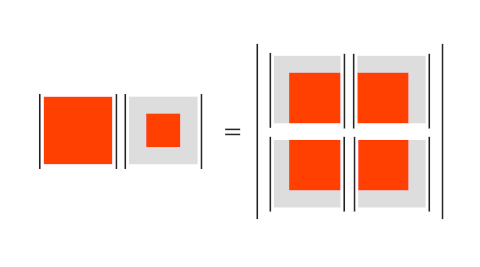
The left side of the image represents the product of two determinants, a full k × k matrix and the k−2 × k−2 matrix formed by removing the edges of the matrix.

The right side of the image is a 2 × 2 determinant who entries are themselves determinants. The four k−1 × k−1 matrices on the right are formed by stripping off the outside row and column of each matrix.

Here’s a demonstration of the identity using the matrix from the example in the previous post and Mathematica.

    a = Det[{{3, 1, 4, 1}, {5, 9, 2, 6}, {0, 7, 1, 0}, {2, 0, 2, 3}}];
    b = Det[{{9, 2}, {7, 1}}];
    c = Det[{{9, 2, 6}, {7, 1, 0}, {0, 2, 3}}];
    d = Det[{{5, 9, 2}, {0, 7, 1}, {2, 0, 2}}];
    e = Det[{{1, 4, 1}, {9, 2, 6}, {7, 1, 0}}];
    f = Det[{{3, 1, 4}, {5, 9, 2}, {0, 7, 1}}];

    a b == c f - d e
    True