The Mersenne Twister (MT) is a random number generator with good statistical properties but bad cryptographic properties. In buzzwords, it’s a PRNG but not a CSPRNG.
This post will show how the internal state of a MT generator can be recovered from its output. We’ll do this using linear algebra. The bit twiddling approach is more common and more efficient, but the linear algebra approach is conceptually simpler.
How MT works
There are numerous variations on the Mersenne Twister. We’ll focus on the original version that had internal state consists of vector x of length 640 filled with 32-bit numbers. The ideas in this post would apply equally to all MT versions.
The first call to MT returns a “tempered” version of x[0]. The next call returned a tempered version of x[1], and so on. After every 640 calls, the state is scrambled. This scrambling is where the “twist” in the name Mersenne Twister comes from. (The Mersenne part comes from the fact that the period of an MT generator is a Mersenne prime.)
Tempering
Here is Python code for performing the tempering step.
def temper(y):
    y ^= (y >> 11)
    y ^= (y <<  7) & 0x9d2c5680
    y ^= (y << 15) & 0xefc60000
    y ^= (y >> 18)
    return y
Each step is reversible, and so the temper function is reversible.
Because the tempering step is reversible, the first output can be used to infer the first element of the internal state, the second output to infer the second element, and so on. After 640 calls one can know the entire internal state and predict the rest of the generator’s output from then on.
Linear algebra
The bitwise operations above all correspond to linear operations over GF(2), the field with just two elements, 0 and 1. Addition in this field is XOR and multiplication is AND.
Each step corresponds to multiplying a vector of 32 bits on the left by a 32 × 32 matrix with entries that are 0’s and 1’s, with the understanding that the sum of two bits is their XOR and the product of two bits is their AND. Equivalently, arithmetic is carried out mod 2. So you can compute the matrix-vector product as ordinary integers if you then reduce every integer mod 2.
We will find the matrix M that corresponds to the temper operation and prove that it is invertible by finding its inverse. This proves that tempering is invertible, and one could compute the inverse of tempering by multiplying by M−1, though it would be more efficient to undo tempering by bit twiddling.
One way to recover a matrix is to multiplying by unit vectors ei where the ith component of ei is 1 and the rest of the components are zero. Then
M ei
is the ith column of M.
So we can find the nth column of M by tempering 1 << n = 2n.
M = np.zeros((32, 32), dtype=int)
for i in range(32):
    t = temper(1 << (31-i))
    s = f"{t:032b}"
    for j in range(32):
        M[j, i] = int(s[j])
Let’s generate a random number and compute its tempered form two ways: directly and matrix multiplication.
x = random.getrandbits(32)
y = temper(x)
print(f"{y:032b}")

vx = np.array([int(b) for b in f"{x:032b}"]) # vector form of x
vy = M @ vx % 2 # vector form of y
print("".join(str(b) for b in vy))
Both produce the same bits:
10100101100101101100110101000110
10100101100101101100110101000110
We can find the matrix representation of the untemper function by inverting the matrix M. However, we need to invert it over the field GF(2), not over the integers or reals.
import galois
GF2 = galois.GF(2)
Minv = np.linalg.inv(GF2(M))
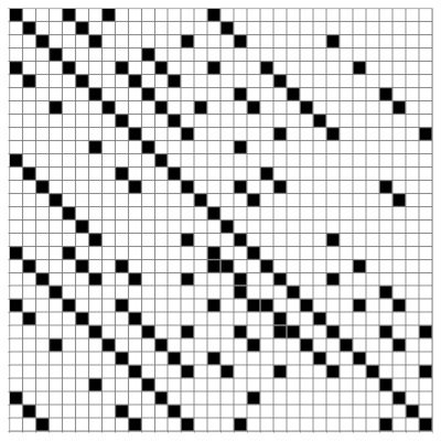
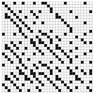
Here are visualizations of M and its inverse using a black square for a 1 and a white square for a 0.
M:
M−1:
The next post will back up and look at the linear algebra of the components that comprise the Mersenne Twister.
![\left[ \begin{array}{cc|cc|cc|c} 0 & -1 & 0 & 0 & 0 & 0 & \cdots \\ 1 & 0 & 0 & 0 & 0 & 0 & \cdots \\ \hline 0 & 0 & 0 & -1 & 0 & 0 & \cdots \\ 0 & 0 & 1 & 0 & 0 & 0 & \cdots \\ \hline 0 & 0 & 0 & 0 & 0 & -1 & \cdots \\ 0 & 0 & 0 & 0 & 1 & 0 & \cdots \\ \hline \vdots & \vdots & \vdots & \vdots & \vdots & \vdots & \ddots \end{array} \right] \left[ \begin{array}{c} a_1 \\ b_1 \\ \hline a_2 \\ b_2 \\ \hline a_3 \\ b_3 \\ \hline \vdots \end{array} \right]](https://www.johndcook.com/hilbert_transform_matrix.svg)