How Mathematica Draws a Dragonfly

Mathematica includes code to draw various whimsical images. For example, if you enter the following command in Mathematica

    Entity["PopularCurve", "DragonflyCurve"][
        EntityProperty["PopularCurve", "Image"]]

you get an image of a dragonfly.

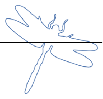
It draws such images with Fourier series. You can tell by asking for the parameterization of the curve. If you enter

    Entity["PopularCurve", "DragonflyCurve"][
        EntityProperty["PopularCurve", "ParametricEquations"]]

you’ll get the following, after some rearrangement.

    Function[t, {
        (7714/27) Sin[47/20 - t] + (1527/37) Sin[16/5 - 2t] + 
        (3202/39) Sin[108/41 - 3t] + … + 2/9 Sin[15/19 - 81 t], 
        (9406/37) Sin[29/7 - t] + (3591/53) Sin[28/13 - 2t] + 
        (1111/20) Sin[9/23 - 3t] + … -(3/29) Sin[8/23 + 81 t]
        }]

The function is a parameterized curve, taking t to (x(t), y(t)) where x(t) and y(t) are Fourier series including frequencies up to sin(81t). Each of the sine terms has a phase shift that could be eliminated by expressing sin(φ + ωt) as a linear combination of sin(ωt) and cos(ωt).

Presumably somebody drew the dragonfly, say in Adobe Illustrator or Inkscape, then did a Fourier transform of a sampling of the curve.

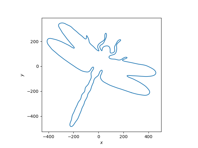
To make sure Mathematica wasn’t doing anything behind the scenes that I wasn’t aware of, I reproduced the dragonfly curve by porting the Mathematica code to Python.

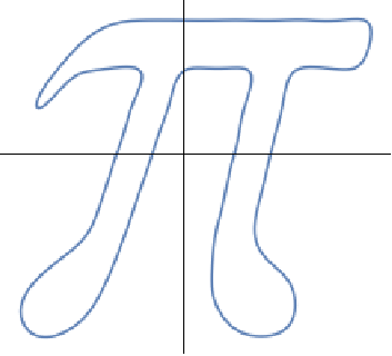
The number of Fourier components needed to draw an image depends on the smoothness and complexity of the image. The curve for π, for example, the highest frequency component is sin(32t).

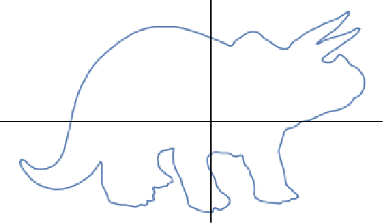
The triceratops curve is more complicated and Mathematica uses frequencies up to sin(188t).